废话不多说,直接上代码!
重要的部分有注释,所有的参数都有参数说明,可以直接运行,适合小白。
转自本人的知乎文章:
https://zhuanlan.zhihu.com/p/271043446
未经许可,禁止转载。
#1、使用sklearn自带的红酒数据集
from sklearn import tree
from sklearn.datasets import load_wine
from sklearn.model_selection import train_test_split
#2、加载数据
wine = load_wine()
#3、随机选70%为训练集,30%为测试集
Xtrain, Xtest, Ytrain, Ytest = train_test_split(
wine.data
,
wine.target
,test_size=0.3)
#4、建立模型,参数选用的是最常见的
clf = tree.DecisionTreeClassifier(criterion=”entropy”
,random_state=7
,splitter=”best”
,max_depth=3
,min_samples_leaf=10
,min_samples_split=10
)
#参数说明:
#criterion:entropy或者gini;
#random_state:随机数种子,不断调整random_state,使分数score变到最高为止;
#splitter有”best”和”random”两种选择,默认值是best,best是优先选择更重要的特征进行分枝,random是分枝时会更加随机,防止过拟合的一种方式,树会变宽变深
#max_depth=3代表限制树的最大高度为3,
#min_samples_leaf=10代表每个结点的样本数量samples最小为10
#min_samples_split=10代表每个非叶结点的样本数量samples最小为10(注意与上一个参数的区别)
clf =
clf.fit
(Xtrain, Ytrain) #代入训练数据
#5、打分并比较
score1 = clf.score(Xtest, Ytest) #代入测试数据,打分,即对训练集的拟合程度
score2 = clf.score(Xtrain, Ytrain) #对训练集的拟合程度如何
#比较score1与score2,如果差距较大,说明过拟合,调整参数splitter,或剪叶参数max_depth(最常用),min_samples_leaf & min_samples_split,max_features & min_impurity_decrease等等
#6、画出树形图
feature_name = [‘酒精’,’苹果酸’,’灰’,’灰的碱性’,’镁’,’总酚’,’类黄酮’,’非黄烷类酚类’,’花青素’,’颜色强度’,’色调’,’稀释葡萄酒’,’脯氨酸’]
import graphviz
dot_data = tree.export_graphviz(clf
,out_file = None
,feature_names= feature_name
,class_names=[“分类1″,”分类2″,”分类3”]
,filled=True
,rounded=True
)
graph = graphviz.Source(dot_data)
graph
#参数说明:
#filled=True ,设置填充颜色,一类一个颜色,从根到叶,颜色逐渐变深;
#rounded=True,设置框的形状
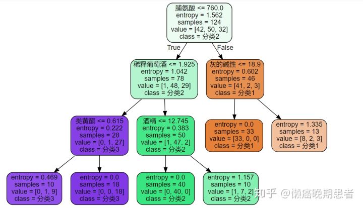
#说明:samples:样本数量,value:每个标签(指标0/1/2)占得样本数量,entropy从根到叶逐渐降低,当entropy为0代表此时可选出一个类别了
#7、其他工作
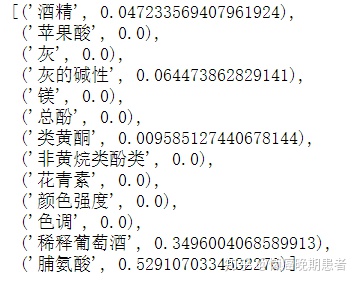
#7.1、上述决策树并没有用到全部的属性
clf.feature_importances_ #查看每个属性的重要/贡献程度,越大越好(根节点贡献程度最高)
[*zip(feature_name,clf.feature_importances_)] #同上,只不过更清晰
#7.2、使用画图的方法确认最优的剪枝参数,一次只能确定一个参数,如确定最优的max_depth:
import matplotlib.pyplot as plt
test = []
for i in range(10):
clf = tree.DecisionTreeClassifier(max_depth=i+1
,criterion=”entropy”
,random_state=30
,splitter=”random”
)
clf =
clf.fit
(Xtrain, Ytrain)
score = clf.score(Xtest, Ytest)
test.append(score)
#针对 max_depth 和 测试集的分数 画图
plt.plot(range(1,11),test,color=”red”,label=”max_depth”)
plt.legend()
plt.show
()
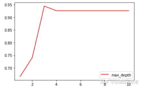
#可以看到max_depth=3时score最高