机器人运动估计——IMU运动方程与ESKF原理介绍（下）

Hello! 欢迎来到我的博客
今天的内容关于机器人中常用的传感器IMU，我们用它来实现机器人姿态、速度、位置的估计。
今天将会介绍使用低成本IMU进行机器人运动估计的一个常用方法——ESKF。

3 Error State Kalman Filter（ESKF介绍）

3.1 动机与流程

使用IMU的初衷是为了求解载体的位置、速度、姿态等系统状态，然而由于IMU测量数据（包括加速度计和陀螺仪的测量数据）都带有大量噪声，直接利用IMU运动方程进行积分会随着时间发生显著的漂移。因此，为了避免漂移我们需要融合其他传感器的信息（如GPS、视觉），对IMU运动积分的结果进行修正。

Error-state Kalman Filter（ESKF）就是一种传感器融合的算法，它的基础仍然是卡尔曼滤波。它的核心思想是把系统的状态分为三类：

true state：实际状态，系统实际的运行状态
nominal state：名义状态，描述了运动状态的主要趋势，主导成分。（large-signal，非线性）
error state：误差状态，实际状态与名义状态之间的差值（small-signal，近似线性，适合线性高斯滤波）

基于以上状态分类，我们可以将关心的true-state，分为两部分，分别进行估计，即nominal state和error state，然后再进行二者叠加。

ESKF的全过程可以描述为如下步骤：

对高频率的IMU数据 $\mathbf{u}_m um进行积分，获得nomimal state x \mathbf{x} x。（注意：nominal state里面不考虑噪声，因此势必会累积误差。这部分误差可依据error state进行修正）$
利用Kalman Filter估计error state，这里同样也包括时间更新和量测更新两部分。（注意：这个过程考虑了噪声，并且由于误差状态方程是近似线性的，所以可以直接用卡尔曼滤波）
利用error state修正nominal state，获取true state
重置error state

使用ESKF的优势：

error state 中的参数数量与运动自由度是相等的，避免了过参数化（over-parameterization or redundancy）引起的协方差矩阵奇异的风险。
error state 总是接近于0，Kalman Filter工作在原点附近。因此，远离奇异值、万向节锁，并且保证了线性化的合理性和有效性。
error state 总是很小，因此二阶项都可以忽略，因此雅可比矩阵的计算会很简单，很迅速。
error state 的变化平缓，因此KF修正的频率不需要太高。

3.2 状态定义

所有在ESKF中用到的变量定义如下：
在这里插入图片描述
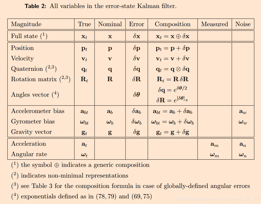
图片中定义了所以状态，包括true state，nominal state以及error state。以及error state和nominal state组合获得true state的方式。
另外，图中的各个运算符在上一篇文章中均已有了定义。除了一个叉乘矩阵的符号，其定义如下：

[

]

≜

[

−

]

[\mathbf{a}]_{\times} \triangleq\left[\begin{array}{ccc} 0 & -a_{z} & a_{y} \\ a_{z} & 0 & -a_{x} \\ -a_{y} & a_{x} & 0 \end{array}\right]

$[a]_{\times} ≜ ⎣ ⎡ 0 a_{z} - a_{y} - a_{z} 0 a_{x} a_{y} - a_{x} 0 ⎦ ⎤$

图片来自于参考文献[1]的P31。

3.3 Nominal State 积分更新（每个时间步都要执行）

3.3.1 Nominal state 方程（连续时间）：

(

−

)

⊗

(

−

)

\begin{aligned} \dot{\mathbf{p}} &=\mathbf{v} \\ \dot{\mathbf{v}} &=\mathbf{R}\left(\mathbf{a}_{m}-\mathbf{a}_{b}\right)+\mathbf{g} \\ \dot{\mathbf{q}} &=\frac{1}{2} \mathbf{q} \otimes\left(\bm\omega_{m}-\bm\omega_{b}\right) \\ \dot{\mathbf{a}}_{b} &=0 \\ \dot{\bm\omega}_{b} &=0 \\ \dot{\mathbf{g}} &=0 \end{aligned}

$\dot{p} \dot{v} \dot{q} \dot{a}_{b} \dot{ω}_{b} \dot{g} = v = R (a_{m} - a_{b}) + g = \frac{1}{2} q \otimes (ω_{m} - ω_{b}) = 0 = 0 = 0$

其中，

{

}

\mathbf{R}=\mathbf{R}\{\mathbf{q}\}

$R = R {q}$ 是基于

\mathbf{q}

$q$ 生成的旋转矩阵，表示从IMU系到惯性系的旋转。
注意到，这组方程完全没有考虑噪声。这组方程的推导是显而意见的，只需要在IMU运动方程的基础上，假设噪声项全部为0即可。

3.3.2 Nominal state 方程（离散时间，用于写程序）：

←

(

−

)

←

(

−

)

←

⊗

{

(

−

)

}

←

\begin{array}{l} \mathbf{p} \leftarrow \mathbf{p}+\mathbf{v} \Delta t+\frac{1}{2}\left(\mathbf{R}\left(\mathbf{a}_{m}-\mathbf{a}_{b}\right)+\mathbf{g}\right) \Delta t^{2} \\ \mathbf{v} \leftarrow \mathbf{v}+\left(\mathbf{R}\left(\mathbf{a}_{m}-\mathbf{a}_{b}\right)+\mathbf{g}\right) \Delta t \\ \mathbf{q} \leftarrow \mathbf{q} \otimes \mathbf{q}\left\{\left(\bm\omega_{m}-\bm\omega_{b}\right) \Delta t\right\} \\ \mathbf{a}_{b} \leftarrow \mathbf{a}_{b} \\ \bm\omega_{b} \leftarrow \bm\omega_{b} \\ \mathbf{g} \leftarrow \mathbf{g} \end{array}

$p \leftarrow p + v Δ t + \frac{1}{2} (R (a_{m} - a_{b}) + g) Δ t^{2} v \leftarrow v + (R (a_{m} - a_{b}) + g) Δ t q \leftarrow q \otimes q {(ω_{m} - ω_{b}) Δ t} a_{b} \leftarrow a_{b} ω_{b} \leftarrow ω_{b} g \leftarrow g$
其中，定义

{

}

\mathbf{q}\left\{\mathbf{v}\right\}=e^{\mathbf{v} / 2}

$q {v} = e^{v / 2}$ ，所以：

{

(

−

)

}

(

−

)

[

cos

⁡

(

)

sin

⁡

(

)

]

\mathbf{q}\left\{\left(\bm\omega_{m}-\bm\omega_{b}\right) \Delta t\right\}=e^{\mathbf{\left(\bm\omega_{m}-\bm\omega_{b}\right) \Delta t} / 2}=e^{\mathbf{u}\theta/ 2}= \left[\begin{array}{c} \cos (\theta/ 2) \\ \mathbf{u} \sin (\theta/ 2) \end{array}\right]

$q {(ω_{m} - ω_{b}) Δ t} = e^{(ω_{m} - ω_{b}) Δ t / 2} = e^{u θ / 2} = [cos (θ / 2) u sin (θ / 2)]$
其中，

∣

(

−

)

∣

(

−

)

\theta=||\left(\bm\omega_{m}-\bm\omega_{b}\right) \Delta t||,\mathbf{u}=\frac{\left(\bm\omega_{m}-\bm\omega_{b}\right) \Delta t}{\theta}

$θ = ∣ ∣ (ω_{m} - ω_{b}) Δ t ∣ ∣, u = \frac{( ω _{m} - ω _{b} ) Δ t}{θ}$

实际上，上面这个操作就是把角度增量改造成单位四元数，两个单位四元数相乘仍然是单位四元数，这样才能保证

q

\mathbf{q}

$q$ 始终为单位四元数，保证迭代是收敛的。

3.4 Error State 时间更新（每个时间步都要执行）

3.4.1 Error state 方程（连续时间）：

−

[

−

]

−

[

−

]

−

\begin{aligned} \delta \dot\mathbf{p} &=\delta \mathbf{v} \\ \dot{\delta \mathbf{v}} &=-\mathbf{R}\left[\mathbf{a}_{m}-\mathbf{a}_{b}\right]_{\times} \delta \boldsymbol{\theta}-\mathbf{R} \delta \mathbf{a}_{b}+\delta \mathbf{g}-\mathbf{R} \mathbf{a}_{n} \\ {\delta} \dot\boldsymbol{\theta} &=-\left[\boldsymbol{\omega}_{m}-\boldsymbol{\omega}_{b}\right]_{\times} \delta \boldsymbol{\theta}-\delta \boldsymbol{\omega}_{b}-\boldsymbol{\omega}_{n} \\ \delta\dot \mathbf{a}_{b} &=\mathbf{a}_{w} \\ \delta \dot{\boldsymbol{\omega}}_{b} &=\boldsymbol{\omega}_{w} \\ \dot{\delta \mathbf{g}} &=0 \end{aligned}

$δ \dot{p} \dot{δ v} δ \dot{θ} δ \dot{a}_{b} δ \dot{ω}_{b} \dot{δ g} = δ v = - R [a_{m} - a_{b}]_{\times} δ θ - R δ a_{b} + δ g - R a_{n} = - [ω_{m} - ω_{b}]_{\times} δ θ - δ ω_{b} - ω_{n} = a_{w} = ω_{w} = 0$
这个误差方程，考虑了噪声等不确定性。其形式看起来似乎不太直观，但实际上推导也很简单。
比如，以位置为例：

−

\delta \mathbf{p}=\mathbf{p}_t-\mathbf{p}

$δ p = p_{t} - p$
所以其导数为：

−

\delta \dot\mathbf{p}=\dot\mathbf{p}_t-\dot\mathbf{p}=\mathbf{v}_t-\mathbf{v}=\delta \mathbf{v}

$δ \dot{p} = \dot{p}_{t} - \dot{p} = v_{t} - v = δ v$
再比如以速度为例：

−

\delta \mathbf{v}=\mathbf{v}_t-\mathbf{v}

$δ v = v_{t} - v$
所以其导数为：

−

(

−

)

−

(

−

)

(

−

)

(

−

)

−

(

)

(

−

)

≈

[

(

[

]

)

−

]

(

−

)

−

(

[

]

)

(

)

≈

[

]

(

−

)

−

(

)

−

[

−

]

−

\begin{aligned} \delta \dot\mathbf{v}&=\dot\mathbf{v}_t-\dot\mathbf{v}\\ &=\mathbf{R}_{t}\left(\mathbf{a}_{m}-\mathbf{a}_{b t}-\mathbf{a}_{n}\right)+\mathbf{g}_{t}-(\mathbf{R}\left(\mathbf{a}_{m}-\mathbf{a}_b\right)+\mathbf{g})\\ &=(\mathbf{R}\delta\mathbf{R}-\mathbf{R})(\mathbf{a}_{m}-\mathbf{a}_{b})-\mathbf{R}\delta\mathbf{R}(\delta\mathbf{a}_b+\mathbf{a}_m)+(\mathbf{g}_t-\mathbf{g})\\ &\approx[\mathbf{R}(\mathbf{I}+[\delta\bm{\theta}]_\times)-\mathbf{R}](\mathbf{a}_{m}-\mathbf{a}_{b})-\mathbf{R}(\mathbf{I}+[\delta\bm{\theta}]_\times)(\delta\mathbf{a}_b+\mathbf{a}_m)+\delta\mathbf{g}\\ &\approx\mathbf{R}[\delta\bm{\theta}]_\times(\mathbf{a}_{m}-\mathbf{a}_{b})-\mathbf{R}(\delta\mathbf{a}_b+\mathbf{a}_m)+\delta\mathbf{g}\\ &=-\mathbf{R}\left[\mathbf{a}_{m}-\mathbf{a}_{b}\right]_{\times} \delta \boldsymbol{\theta}-\mathbf{R} \delta \mathbf{a}_{b}+\delta \mathbf{g}-\mathbf{R} \mathbf{a}_{n} \\ \end{aligned}

$δ \dot{v} = \dot{v}_{t} - \dot{v} = R_{t} (a_{m} - a_{b t} - a_{n}) + g_{t} - (R (a_{m} - a_{b}) + g) = (R δ R - R) (a_{m} - a_{b}) - R δ R (δ a_{b} + a_{m}) + (g_{t} - g) \approx [R (I + [δ θ]_{\times}) - R] (a_{m} - a_{b}) - R (I + [δ θ]_{\times}) (δ a_{b} + a_{m}) + δ g \approx R [δ θ]_{\times} (a_{m} - a_{b}) - R (δ a_{b} + a_{m}) + δ g = - R [a_{m} - a_{b}]_{\times} δ θ - R δ a_{b} + δ g - R a_{n}$
其中，用到了

[

]

≈

[

]

\delta\mathbf{R}=e^{[\delta\bm{\theta}]_\times} \approx \mathbf{I}+[\delta\bm{\theta}]_\times

$δ R = e^{[δ θ]_{\times}} \approx I + [δ θ]_{\times}$ 。此外，还用到了两个小量相乘可以忽略的假设。

其它方程的推导，就不在此说明了，可以参考文献[1]的P33页。

3.4.2 Error state 方程（离散时间，用于写程序）：

定义状态向量：

[

]

∈

[

]

∈

[

]

∈

[

]

∈

\mathbf{x}=\left[\begin{array}{l} \mathbf{p} \\ \mathbf{v} \\ \mathbf{q} \\ \mathbf{a}_{b} \\ \boldsymbol{\omega}_{b} \\ \mathbf{g} \end{array}\right] \in \mathbb{R}_{19\times 1}, \quad \delta \mathbf{x}=\left[\begin{array}{c} \delta \mathbf{p} \\ \delta \mathbf{v} \\ \delta \boldsymbol{\theta} \\ \delta \mathbf{a}_{b} \\ \delta \boldsymbol{\omega}_{b} \\ \delta \mathbf{g} \end{array}\right] \in \mathbb{R}_{18\times 1}\quad, \quad \mathbf{u}_{m}=\left[\begin{array}{c} \mathbf{a}_{m} \\ \boldsymbol{\omega}_{m} \end{array}\right] \in \mathbb{R}_{6\times 1}, \quad \mathbf{i}=\left[\begin{array}{c} \mathbf{v}_{\mathbf{i}} \\ \boldsymbol{\theta}_{\mathbf{i}} \\ \mathbf{a}_{\mathbf{i}} \\ \boldsymbol{\omega}_{\mathbf{i}} \end{array}\right] \in \mathbb{R}_{12\times 1}

$x = ⎣ ⎢ ⎢ ⎢ ⎢ ⎢ ⎢ ⎡ p v q a_{b} ω_{b} g ⎦ ⎥ ⎥ ⎥ ⎥ ⎥ ⎥ ⎤ \in R_{19 \times 1}, δ x = ⎣ ⎢ ⎢ ⎢ ⎢ ⎢ ⎢ ⎡ δ p δ v δ θ δ a_{b} δ ω_{b} δ g ⎦ ⎥ ⎥ ⎥ ⎥ ⎥ ⎥ ⎤ \in R_{18 \times 1}, u_{m} = [a_{m} ω_{m}] \in R_{6 \times 1}, i = ⎣ ⎢ ⎢ ⎡ v_{i} θ_{i} a_{i} ω_{i} ⎦ ⎥ ⎥ ⎤ \in R_{12 \times 1}$
于是误差状态方程可以写作：

←

(

)

(

)

⋅

\delta \mathbf{x} \leftarrow f\left(\mathbf{x}, \delta \mathbf{x}, \mathbf{u}_{m}, \mathbf{i}\right)=\mathbf{F}_{\mathbf{x}}\left(\mathbf{x}, \mathbf{u}_{m}\right) \cdot \delta \mathbf{x}+\mathbf{F}_{\mathbf{i}} \cdot \mathbf{i}

$δ x \leftarrow f (x, δ x, u_{m}, i) = F_{x} (x, u_{m}) \cdot δ x + F_{i} \cdot i$
其中:

∂

∣

[

−

[

−

]

−

⊤

{

(

−

)

}

−

]

∈

\mathbf{F}_{\mathbf{x}}=\left.\frac{\partial f}{\partial \delta \mathbf{x}}\right|_{\mathbf{x}, \mathbf{u}_{m}}=\left[\begin{array}{cccccc} \mathbf{I} & \mathbf{I} \Delta t & 0 & 0 & 0 & 0 \\ 0 & \mathbf{I} & -\mathbf{R}\left[\mathbf{a}_{m}-\mathbf{a}_{b}\right]_{\times} \Delta t & -\mathbf{R} \Delta t & 0 & \mathbf{I} \Delta t \\ 0 & 0 & \mathbf{R}^{\top}\left\{\left(\omega_{m}-\omega_{b}\right) \Delta t\right\} & 0 & -\mathbf{I} \Delta t & 0 \\ 0 & 0 & 0 & \mathbf{I} & 0 & 0 \\ 0 & 0 & 0 & 0 & \mathbf{I} & 0 \\ 0 & 0 & 0 & 0 & 0 & \mathbf{I} \end{array}\right] \in \mathbb{R}_{18\times 18}

$F_{x} = \frac{\partial f}{\partial δ x} ∣ ∣ ∣ ∣_{x, u_{m}} = ⎣ ⎢ ⎢ ⎢ ⎢ ⎢ ⎢ ⎡ I 00000 I Δ t I 0000 0 - R [a_{m} - a_{b}]_{\times} Δ t R^{⊤} {(ω_{m} - ω_{b}) Δ t} 000 0 - R Δ t 0 I 00 00 - I Δ t 0 I 0 0 I Δ t 000 I ⎦ ⎥ ⎥ ⎥ ⎥ ⎥ ⎥ ⎤ \in R_{18 \times 18}$

∂

∣

[

]

∈

[

]

∈

\mathbf{F}_{\mathbf{i}}=\left.\frac{\partial f}{\partial \mathbf{i}}\right|_{\mathbf{x}, \mathbf{u}_{m}}=\left[\begin{array}{cccc} 0 & 0 & 0 & 0 \\ \mathbf{I} & 0 & 0 & 0 \\ 0 & \mathbf{I} & 0 & 0 \\ 0 & 0 & \mathbf{I} & 0 \\ 0 & 0 & 0 & \mathbf{I} \\ 0 & 0 & 0 & 0 \end{array}\right] \quad \in \mathbb{R}_{18\times 12}, \quad \mathbf{Q}_{\mathbf{i}}=\left[\begin{array}{cccc} \mathbf{V}_{\mathbf{i}} & 0 & 0 & 0 \\ 0 & \mathbf{\Theta}_{\mathbf{i}} & 0 & 0 \\ 0 & 0 & \mathbf{A}_{\mathbf{i}} & 0 \\ 0 & 0 & 0 & \mathbf{\Omega}_{\mathbf{i}} \end{array}\right] \in \mathbb{R}_{12\times 12}

$F_{i} = \frac{\partial f}{\partial i} ∣ ∣ ∣ ∣_{x, u_{m}} = ⎣ ⎢ ⎢ ⎢ ⎢ ⎢ ⎢ ⎡ 0 I 0000 00 I 000 000 I 00 0000 I 0 ⎦ ⎥ ⎥ ⎥ ⎥ ⎥ ⎥ ⎤ \in R_{18 \times 12}, Q_{i} = ⎣ ⎢ ⎢ ⎡ V_{i} 000 0 Θ_{i} 00 00 A_{i} 0 000 Ω_{i} ⎦ ⎥ ⎥ ⎤ \in R_{12 \times 12}$

其中，

\mathbf{v}_{\mathbf{i}},\boldsymbol{\theta}_{\mathbf{i}},\mathbf{a}_{\mathbf{i}},\boldsymbol{\omega}_{\mathbf{i}}

$v_{i}, θ_{i}, a_{i}, ω_{i}$ 代表随机脉冲，他们的均值为0，协方差矩阵为对角阵。
另外，定义：

⊤

{

(

−

)

}

−

[

−

]

−

[

−

]

[

−

]

−

\mathbf{R}^{\top}\left\{\left(\boldsymbol{\omega}_{m}-\boldsymbol{\omega}_{b}\right) \Delta t\right\}=e^{-[\boldsymbol{\omega}_{m}-\boldsymbol{\omega}_{b}]_\times \Delta t}=\mathbf{I}-[\boldsymbol{\omega}_{m}-\boldsymbol{\omega}_{b}]_\times \Delta t+\frac{1}{2}[\boldsymbol{\omega}_{m}-\boldsymbol{\omega}_{b}]_\times^2 \Delta t^2-…

$R^{⊤} {(ω_{m} - ω_{b}) Δ t} = e^{- [ω_{m} - ω_{b}]_{\times} Δ t} = I - [ω_{m} - ω_{b}]_{\times} Δ t + \frac{1}{2} [ω_{m} - ω_{b}]_{\times}^{2} Δ t^{2} - . . .$
这是一个微分方程的闭合解，利用这个解进行递推会更精确。当然，也可以只取前面两项。

3.4.3 对于Error state的卡尔曼滤波器的时间更新（用于写程序）

误差状态更新

←

(

)

⋅

\hat{\delta \mathbf{x}} \leftarrow \mathbf{F}_{\mathbf{x}}\left(\mathbf{x}, \mathbf{u}_{m}\right) \cdot \hat{\delta \mathbf{x}}

$\hat{δ x} \leftarrow F_{x} (x, u_{m}) \cdot \hat{δ x}$
协方差矩阵更新

←

⊤

\mathbf{P} \leftarrow \mathbf{F}_{\mathbf{x}} \mathbf{P} \mathbf{F}_{\mathbf{x}}^{\top}+\mathbf{F}_{\mathbf{i}} \mathbf{Q}_{\mathbf{i}} \mathbf{F}_{\mathbf{i}}^{\top}

$P \leftarrow F_{x} P F_{x}^{⊤} + F_{i} Q_{i} F_{i}^{⊤}$
这个就是很基础的卡尔曼滤波方程了，不了解的可以移步我的博客：
机器人运动估计系列（番外篇）——从贝叶斯滤波到卡尔曼（上）

3.5 Error State 量测更新（只有测量值到来的时间步需要执行）

由于IMU的数据中夹带了大量噪声，我们需要利用更多的传感器的信息，来对状态进行修正。

而这些传感器中常用的组合包括：GPS+IMU，单目视觉+IMU，双目视觉+IMU等。

3.5.1 量测方程

通常，量测方程的基本形式如下：

(

)

\mathbf{y}=h\left(\mathbf{x}_{t}\right)+v

$y = h (x_{t}) + v$
其中

(

)

h()

$h ()$ 是量测函数，与传感器有关。

$v$ 是高斯白噪声，为

∼

{

}

v \sim \mathcal{N}\{0, \mathbf{V}\}

$v \sim N {0, V}$ 。

为了实现量测更新，我们需要求

$h$ 对

\delta \mathbf{x}

$δ x$ 的导数，所以有：

≡

∂

∣

∂

∣

∂

∣

\left.\mathbf{H} \equiv \frac{\partial h}{\partial \delta \mathbf{x}}\right|_{\mathbf{x}}=\left.\left.\frac{\partial h}{\partial \mathbf{x}_{t}}\right|_{\mathbf{x}} \frac{\partial \mathbf{x}_{t}}{\partial \delta \mathbf{x}}\right|_{\mathbf{x}}=\mathbf{H}_{\mathbf{x}} \mathbf{X}_{\delta \mathbf{x}}

$H \equiv \frac{\partial h}{\partial δ x} ∣ ∣ ∣ ∣_{x} = \frac{\partial h}{\partial x _{t}} ∣ ∣ ∣ ∣_{x} \frac{\partial x _{t}}{\partial δ x} ∣ ∣ ∣ ∣_{x} = H_{x} X_{δ x}$
其中

≜

∂

∣

\left.\mathbf{H}_{\mathbf{x}} \triangleq \frac{\partial h}{\partial \mathbf{x}_{t}}\right|_{\mathbf{x}}

$H_{x} ≜ \frac{\partial h}{\partial x _{t}} ∣ ∣ ∣_{x}$ 是量测函数的雅可比矩阵，根据传感器的不同而具有不同形式。

而

≜

∂

∣

\left.\mathbf{X}_{\delta \mathbf{x}} \triangleq \frac{\partial \mathbf{x}_{t}}{\partial \delta \mathbf{x}}\right|_{\mathbf{x}}

$X_{δ x} ≜ \frac{\partial x _{t}}{\partial δ x} ∣ ∣ ∣_{x}$ 则可以表示为：

≜

∂

∣

[

]

[

−

]

\left.\mathbf{X}_{\delta \mathbf{x}} \triangleq \frac{\partial \mathbf{x}_{t}}{\partial \delta \mathbf{x}}\right|_{\mathbf{x}}=\left[\begin{array}{ccc} \mathbf{I}_{6} & 0 & 0 \\ 0 & \mathbf{Q}_{\delta \boldsymbol{\theta}} & 0 \\ 0 & 0 & \mathbf{I}_{9} \end{array}\right], \mathbf{Q}_{\delta \boldsymbol{\theta}}=\frac{1}{2}\left[\begin{array}{ccc} -q_{x} & -q_{y} & -q_{z} \\ q_{w} & -q_{z} & q_{y} \\ q_{z} & q_{w} & -q_{x} \\ -q_{y} & q_{x} & q_{w} \end{array}\right]

$X_{δ x} ≜ \frac{\partial x _{t}}{\partial δ x} ∣ ∣ ∣ ∣_{x} = ⎣ ⎡ I_{6} 00 0 Q_{δ θ} 0 00 I_{9} ⎦ ⎤, Q_{δ θ} = \frac{1}{2} ⎣ ⎢ ⎢ ⎡ - q_{x} q_{w} q_{z} - q_{y} - q_{y} - q_{z} q_{w} q_{x} - q_{z} q_{y} - q_{x} q_{w} ⎦ ⎥ ⎥ ⎤$

关于上式的详细推导，可以参考文献[1]的P39页。

3.5.2 对于Error state的卡尔曼滤波器的量测更新（用于写程序）

卡尔曼增益的计算

⊤

(

⊤

)

−

\mathbf{K}=\mathbf{P} \mathbf{H}^{\top}\left(\mathbf{H} \mathbf{P} \mathbf{H}^{\top}+\mathbf{V}\right)^{-1}

$K = P H^{⊤} (H P H^{⊤} + V)^{- 1}$
误差状态量测更新

←

(

−

(

)

\hat{\delta} \mathbf{x} \leftarrow \mathbf{K}\left(\mathbf{y}-h\left(\hat{\mathbf{x}}_{t}\right)\right)

$\hat{δ} x \leftarrow K (y - h (\hat{x}_{t}))$
协方差矩阵更新

←

(

−

)

\mathbf{P} \leftarrow(\mathbf{I}-\mathbf{K} \mathbf{H}) \mathbf{P}

$P \leftarrow (I - K H) P$
这是卡尔曼滤波的基础方程，就不做介绍了。

3.6 状态合并以及Error State 重置（在量测更新过后执行）

3.6.1 状态合并

这一步是要把error state与nominal state合并，即修正nominal state随时间的漂移。

←

⊕

\mathbf{x} \leftarrow \mathbf{x} \oplus \hat{\delta \mathbf{x}}

$x \leftarrow x \oplus \hat{δ x}$
即：

←

⊗

{

}

←

\begin{aligned} &\begin{array}{l} \mathbf{p} \leftarrow \mathbf{p}+\hat{\delta \mathbf{p}} \\ \mathbf{v} \leftarrow \mathbf{v}+\hat{\delta \mathbf{v}} \end{array}\\ &\mathbf{q} \leftarrow \mathbf{q} \otimes \mathbf{q}\{\hat{\delta \boldsymbol{\theta}}\}\\ &\mathbf{a}_{b} \leftarrow \mathbf{a}_{b}+\delta \hat{\mathbf{a}}_{b}\\ &\bm\omega_{b} \leftarrow \bm\omega_{b}+\delta \hat{\bm\omega}_{b}\\ &\mathbf{g} \leftarrow \mathbf{g}+\hat{\delta \mathbf{g}} \end{aligned}

$p←p+δp^v←v+δv^q←q⊗q{δθ^}ab←ab+δa^bωb←ωb+δω^bg←g+δg^$

3.6.2 Error state 重置

由于nominal state的误差已经修正了，所以error state要置零，同时协方差矩阵也要相应的修改。

通常来说，重置的方法如下：

←

⊤

\begin{aligned} &\hat{\delta \mathbf{x}} \leftarrow 0\\ &\mathbf{P} \leftarrow \mathbf{G} \mathbf{P} \mathbf{G}^{\top} \end{aligned}

$\hat{δ x} \leftarrow 0 P \leftarrow G P G^{⊤}$
其中：

\mathbf{G}= \mathbf{I}_{18}

$G = I_{18}$ 。

4 Matlab代码

https://github.com/CASIA-RoboticFish/FBUS-EKF

参考文献

[1] Joan Sol`a. Quaternion kinematics for the error-state KF. Sep 12, 2016.

关于<IMU运动方程与ESKF原理介绍>的上下两篇文章主要内容出自上面这篇参考文献，我只是进行了翻译和重新梳理逻辑顺序的工作。因此，大家如果使用到本博客内容，也烦请引用上述参考文献。谢谢~

原文链接：https://blog.csdn.net/handsome_for_kill/article/details/105189891