首先罗列出文献中总结的以下几个结论:
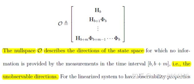
- 能观性矩阵的零空间维度反映了系统不可观的维度
- VINS系统不可观维度等于4,通常为平移和绕重力方向的yaw
- 能观不一致性的原因是EKF的转移和观测Jacobian矩阵的线性化点不同而造成的
- EKF错误的可观现象导致yaw的协方差较小,从而系统整体更新出现累计误差
能观性和相应的解决方法已经有很多作者都进行了分析和求解,本文主要介绍黄国权,Roumeliotis和李明杨三个作者从各自的角度阐述上述问题。
一. 能观性分析和解决方法
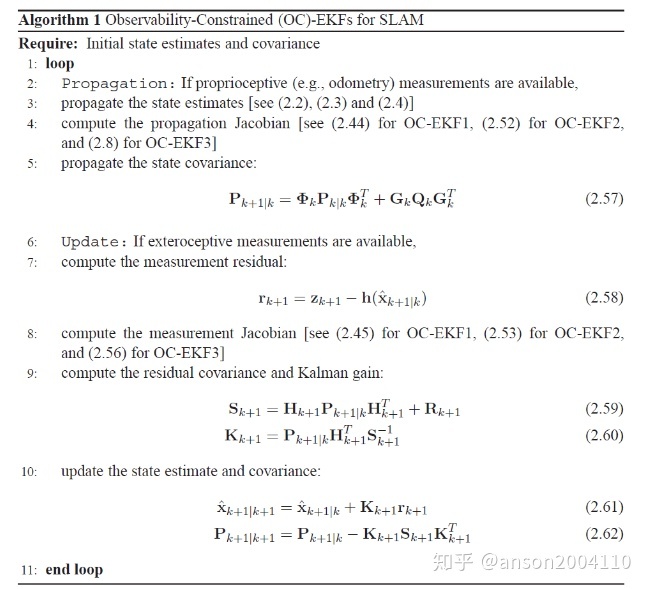
1. OC-EKF, Huangguoquan
step1 首先定义标准的EKF过程如下:
a.定义EKF状态
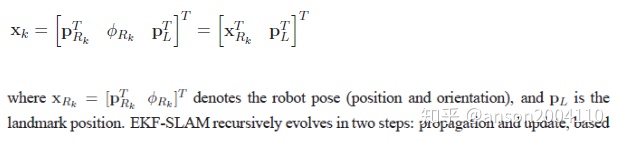
b.定义EKF运动方程
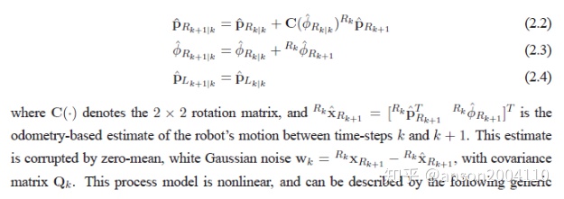
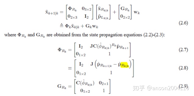
c.定义误差的转移方程
注意这里的pRk|k 表示的是上一时刻的EKF状态更新值
d. 测量更新
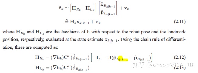
注意这里的pLk|k-1 表示的是上一时刻的EKF状态估计值
step 2 分析一个非线性SLAM系统的不可观维度,如2D SLAM系统如下:
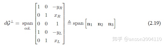
可见,零空间的维度=3,旋转θ和平移量xy不可观
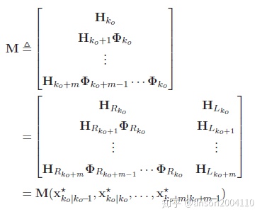
step 3 构造EKF线性化系统的能观性矩阵
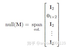
step 4 对于理想EKF系统的情况下,假设真值已知,且
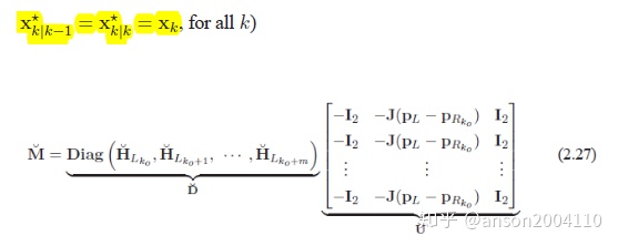
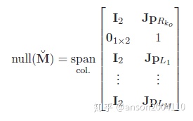
零空间的维度仍然为3
step 5 对于实际EKF系统的情况下,真值未知,且
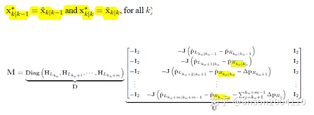
可见,实际EKF系统的能观性矩阵零空间的维度为2
可见,不同的线性化点对于系统可观性的影响,文章原话如下:
In turn, this implies that the choice of linearization points affects the observability properties of the linearized error-state system of the EKF.
这一现象导致系统认为旋转量被错误的可观,从而协方差较小,可信度较高,对其更新量较小,从而导致旋转方向上的误差累计越来越多,整个系统的误差水平也越来越大。
解决上述的能观性不一致的思路,需要满足
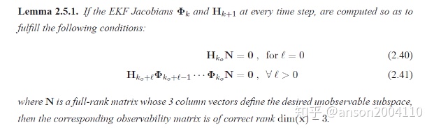
即,在每次的EKF传递和更新过程中,保证N空间的维度始终等于3
step 6 解决方案1,OC-EKF1,也就是First-Estimates-Jacobian (FEJ)-EKF
这个方法直接用上一时刻的估计值替换EKF上一时刻的预测值,带入到转移和观测矩阵
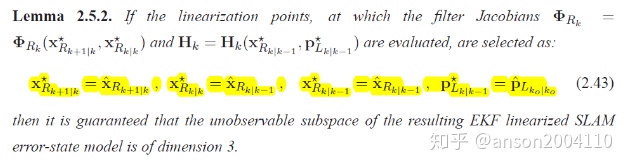
替换
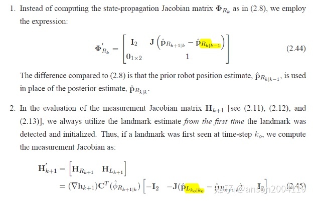
step 7 解决方案2,OC-EKF2
方法一的精度和稳定性取决于 线性化点估计值的准确性
Even though the OC-EKF1 typically performs substantially better than the standard EKF (see Sections 2.6 and 2.7), it relies heavily on the initial state estimates; if these estimates are inaccurate, the linearization errors become large and thus the performance of the estimator may
degrade. This could be the case when the first estimates of the landmark positions are of poor quality (e.g., in bearing-only SLAM).
所以作者提出了一种已知条件的优化问题
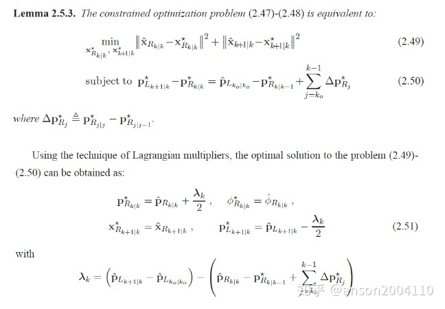
拉格朗日乘子法(Lagrange Multiplier)参考https://blog.csdn.net/zhangyingjie09/article/details/80368494
已知了λ之后,可以对转移和观测矩阵进行调整:
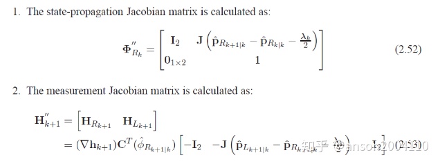
step 8 解决方案3,OC-EKF3
与OC-EKF2先求取线性化点的变量,再求取转移和观测矩阵不同,该方法直接计算观测矩阵
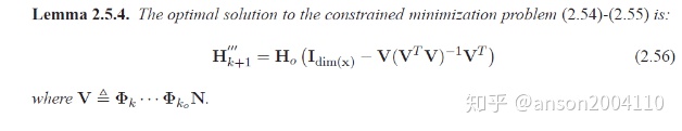
上述三种方案总结如下:
参考:
2008 Analysis and improvement of the consistency of extended kalman filter based slam
2010 Observability-based Rules for Designing Consistent EKF SLAM Estimators.
博士论文 Improving the Consistency of Nonlinear Estimators Analysis Algorithms and Applications
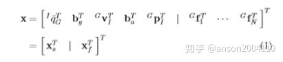
2. OC-VINS,Stergios I. Roumeliotis
这个能观性分析和调整方法用在了kumar s-MSCKF中,对转移和观测矩阵进行调整。同时,注意到他也将特征点分成跟踪OF和SLAM特征点DF。
step 1 定义EKF状态(除了IMU的状态之外,还含有SLAM特征点坐标,IMU状态用MSCKF的方法来更新,SLAM特征点用EKF的方法来更新)
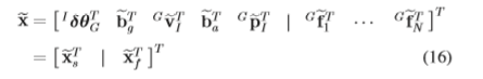
step 2 定义 EKF误差状态
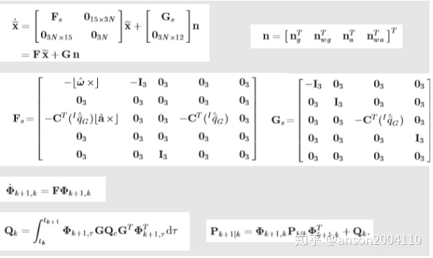
step 3 EKF状态转移和协方差矩阵
step 4 EKF 观测矩阵

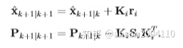
step 5 EKF 残差和权值
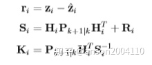
step 6 EKF更新
step 7 定义能观性矩阵
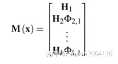
step 8 带入转移和观测矩阵
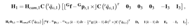
step 9 零空间分析
为了保证能观一致性,需要满足
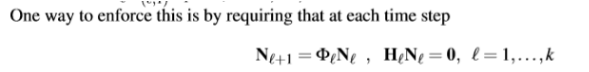
注,与huangguoquan的能观性修正方法的思路一致,都是要满足上述公式,只不过具体求解转移和观测矩阵的封闭解过程不同。
step 10 调整转移矩阵
已知
则
非零的三行写成:
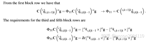
上述三个式子构成了拉格朗日乘法优化目标函数:
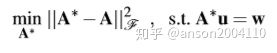
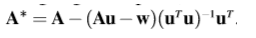
求解
step 11 调整观测矩阵
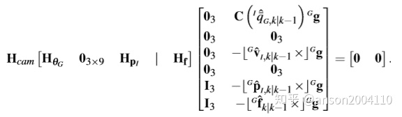
则
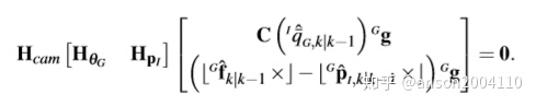
上述两个式子构成了拉格朗日乘法优化目标函数:
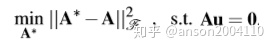
求解A*并且更新H

参考:
2012 Observability-constrained vision-aided inertial navigation
2014 Consistency analysis and improvement of vision-aided inertial navigation
3. MSCKF2.0, limingyang
step 1 分析非线性系统,如一个典型的运动和观测系统
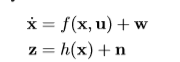
用EKF线性化操作近似后
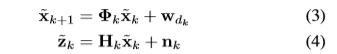
能观性不一致性的原因是因为Jacobian求导(用了不同的线性化点),原本yaw 不可观,变成可观,从而估计器的协方差很小,导致整个系统更新不正确。原文如下
EKF: we prove that, due to the way the EKF Jacobians are computed, even though the IMU’s rotation about gravity (the yaw) is not observable in VIO, it appears to be observable in the linearized system model used by the MSCKF { and the same occurs in EKF-SLAM. Thus, the estimator erroneously believes it has more information than it actually does, and reports a covariance matrix for the state that underestimates the actual one.
Specically, due to the way in which the Jacobians are computed in the EKF, the global orientation appears to be observable in the linearized model, while it is not in the actual system. As a result of this mismatch, the lter produces too small values for the state covariance matrix.
step 2 构造能观性矩阵
step 3 求取转移矩阵
已知旋转误差项的左乘公式
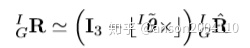
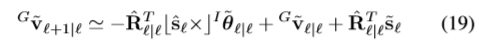
则,IMU旋转的误差传递关系如下
则
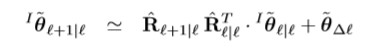
速度的误差传递关系
位置的误差传递关系

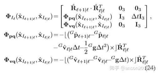
整理得到:
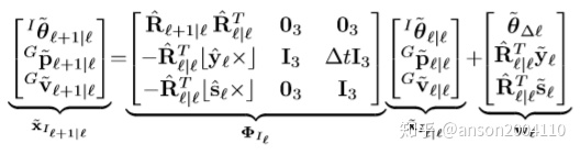
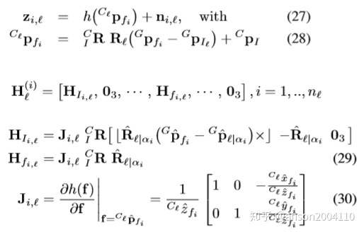
step 4 求取观测矩阵
观测矩阵
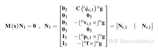
step 5 构造能观性矩阵
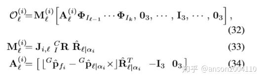
step 6 理想情况下的能观性矩阵和零空间
To derive the “ideal” observability matrix, we evaluate the state transition matrix as Φ(xEk+1; xEk) , and evaluate the Jacobian matrix using the true states.
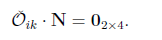
能观性矩阵
零空间
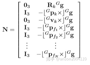
可见,维度=4
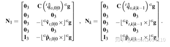
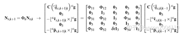
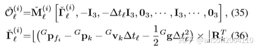
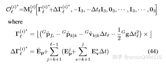
step 7 实际的能观性矩阵和零空间
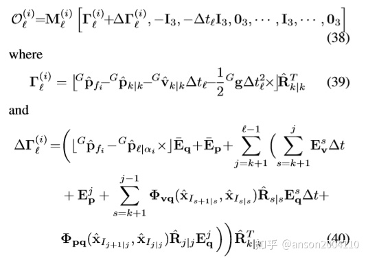
其中
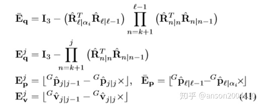
可见,与式35相比,能观性矩阵O 式38中第一项多了一个扰动项ΔΓ,如原文:
The key dierence is that when the Jacobians are evaluated using the state estimates instead of the true states, the disturbance” term ΔΓ appears.
观察这个扰动项中,Eq,Ep和Ev都反映了线性化点不同导致。能观性不一致的原因:
in the original MSCKF dierent estimates of the same states are used for computing Jacobians, and this leads to an infusion of fictitious” information about the yaw. Specically, the use of dierent estimates for the IMU position and velocity result in nonzero values for the disturbance terms ΔΓ, which change the dimension of the nullspace of the observability matrix.
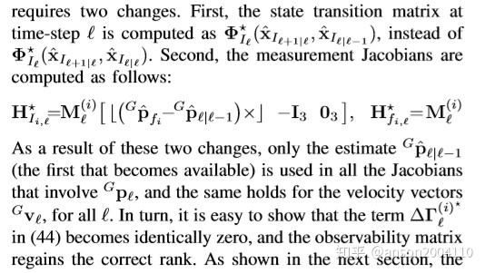
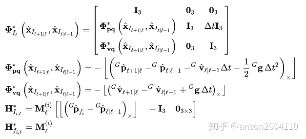
step 7 改进方案
a. 左乘改成“右乘”,调整转移矩阵
这里用了数学上的右乘数值近似,非本质上矩阵的右乘。
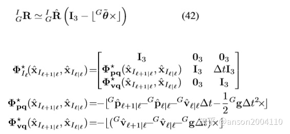
与式24 相比,转移矩阵中与R相关的都去除了。且,观测矩阵仍然为
带入能观性矩阵,得
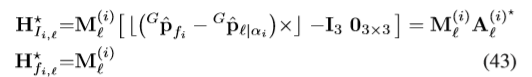
b. FEJ
为了消除上述遇到的Ep,Eq和Ev。原文如下
则:
参考
2012 Improving the accuracy of ekf-based visual-inertial odometry
2013 High-Precision, Consistent EKF-based Visual-Inertial Odometry
博士论文 Visual-Inertial Odometry on Resource-Constrained Systems
二 . OpenVINS 代码中的FEJ的应用
1 保存状态的估计值
1 在Propagator::predict_and_compute预积分后更新MSCKF的IMU状态
state->imu()->set_value(imu_x);
state->imu()->set_fej(imu_x);
2 初始化 时间偏差,IMU到相机外的参数和相机内参数
state->calib_dt_CAMtoIMU()->set_value(temp_camimu_dt);
state->calib_dt_CAMtoIMU()->set_fej(temp_camimu_dt);
state->get_intrinsics_CAM(i)->set_value(cam_calib);
state->get_intrinsics_CAM(i)->set_fej(cam_calib);
state->get_calib_IMUtoCAM(i)->set_value(cam_eigen);
state->get_calib_IMUtoCAM(i)->set_fej(cam_eigen);
3 在Landmark::set_from_xyz设置特征点(5种不同的情况下)
if(isfej) set_fej(p_FinG);
if(isfej) set_fej(p_invFinG);
if(isfej) set_fej(p_invFinA_MSCKF);
这个函数是在UpdaterSLAM::delayed_init中调用,对长期的slam点更新MSCKF状态之后。
if(FeatureRepresentation::is_relative_representation(feat.feat_representation)) {
landmark->_anchor_cam_id = feat.anchor_cam_id;
landmark->_anchor_clone_timestamp = feat.anchor_clone_timestamp;
landmark->set_from_xyz(feat.p_FinA, false);
landmark->set_from_xyz(feat.p_FinA_fej, true);
} else {
landmark->set_from_xyz(feat.p_FinG, false);
landmark->set_from_xyz(feat.p_FinG_fej, true);
}
UpdaterSLAM::perform_anchor_change(若特征点表示方法是局部的情况下调用)
landmark->set_from_xyz(new_feat.p_FinA, false);
landmark->set_from_xyz(new_feat.p_FinA_fej, true);
4 在UpdaterSLAM::delayed_init取长期的特征点作为更新MSCKF 特征点状态
// Save the position and its fej value
if(FeatureRepresentation::is_relative_representation(feat.feat_representation)) {
feat.anchor_cam_id = (*it2)->anchor_cam_id;
feat.anchor_clone_timestamp = (*it2)->anchor_clone_timestamp;
feat.p_FinA = (*it2)->p_FinA;
feat.p_FinA_fej = (*it2)->p_FinA;
} else {
feat.p_FinG = (*it2)->p_FinG;
feat.p_FinG_fej = (*it2)->p_FinG;
}
5 在UpdaterSLAM::update 取slam 特征点集中的landmark 作为更新MSCKF 特征点状态
// Save the position and its fej value
if(FeatureRepresentation::is_relative_representation(feat.feat_representation)) {
feat.anchor_cam_id = landmark->_anchor_cam_id;
feat.anchor_clone_timestamp = landmark->_anchor_clone_timestamp;
feat.p_FinA = landmark->get_xyz(false);
feat.p_FinA_fej = landmark->get_xyz(true);
} else {
feat.p_FinG = landmark->get_xyz(false);
feat.p_FinG_fej = landmark->get_xyz(true);
}
6 在UpdaterMSCKF::update 取传统的msckf特征点集作为更新MSCKF状态
// Save the position and its fej value
if(FeatureRepresentation::is_relative_representation(feat.feat_representation)) {
feat.anchor_cam_id = (*it2)->anchor_cam_id;
feat.anchor_clone_timestamp = (*it2)->anchor_clone_timestamp;
feat.p_FinA = (*it2)->p_FinA;
feat.p_FinA_fej = (*it2)->p_FinA;
} else {
feat.p_FinG = (*it2)->p_FinG;
feat.p_FinG_fej = (*it2)->p_FinG;
}
7 在UpdaterSLAM::perform_anchor_change 的局部坐标系转换需要设置
old_feat.p_FinA_fej = landmark->get_xyz(true);
new_feat.p_FinA_fej = R_OLDtoNEW_fej*landmark->get_xyz(true)+p_OLDinNEW_fej;
2 求解Φ和H Jacobian矩阵的时候使用
1 在UpdaterHelper::get_feature_jacobian_representation 中获取特征点在世界坐标系下的坐标
// Get the feature linearization point
Eigen::Matrix<double,3,1> p_FinG = (state->options().do_fej)? feature.p_FinG_fej : feature.p_FinG;
2 在UpdaterHelper::get_feature_jacobian_representation 中获取特征点的在局部坐标系的坐标,用到IMU到世界坐标系的关系
// If I am doing FEJ, I should FEJ the anchor states (should we fej calibration???)
// Also get the FEJ position of the feature if we are
if(state->options().do_fej) {
// “Best” feature in the global frame
Eigen::Vector3d p_FinG_best = R_GtoI.transpose() * R_ItoC.transpose()*(feature.p_FinA – p_IinC) + p_IinG;
// Transform the best into our anchor frame using FEJ
R_GtoI = state->get_clone(feature.anchor_clone_timestamp)->Rot_fej();
p_IinG = state->get_clone(feature.anchor_clone_timestamp)->pos_fej();
p_FinA = (R_GtoI.transpose()*R_ItoC.transpose()).transpose()*(p_FinG_best – p_IinG) + p_IinC;
}
3 UpdaterHelper::get_feature_jacobian_full 特征点的在局部or全局坐标系下的表示
// Calculate the position of this feature in the global frame FEJ
// If anchored, then we can use the “best” p_FinG since the value of p_FinA does not matter
Eigen::Vector3d p_FinG_fej = feature.p_FinG_fej;
if(FeatureRepresentation::is_relative_representation(feature.feat_representation)) {
p_FinG_fej = p_FinG;
}
4 UpdaterHelper::get_feature_jacobian_full IMU状态到世界坐标系的关系,特征点分别在IMU和相机坐标系下的坐标
// If we are doing first estimate Jacobians, then overwrite with the first estimates
if(state->options().do_fej) {
R_GtoIi = clone_Ii->Rot_fej();
p_IiinG = clone_Ii->pos_fej();
p_FinIi = R_GtoIi*(p_FinG_fej-p_IiinG);
p_FinCi = R_ItoC*p_FinIi+p_IinC;
}
5 Propagator::predict_and_compute 在更新协方差的时候用到
// Now compute Jacobian of new state wrt old state and noise
if (state->options().do_fej) {
// This is the change in the orientation from the end of the last prop to the current prop
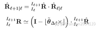
// This is needed since we need to include the “k-th” updated orientation information
Eigen::Matrix<double,3,3> Rfej = state->imu()->Rot_fej();
Eigen::Matrix<double,3,3> dR = quat_2_Rot(new_q)*Rfej.transpose(); 和非FEJ不同,这里求的是imu这一旋转量关于世界坐标系的关系
Eigen::Matrix<double,3,1> v_fej = state->imu()->vel_fej();
Eigen::Matrix<double,3,1> p_fej = state->imu()->pos_fej();
F.block(th_id, th_id, 3, 3) = dR;
F.block(th_id, bg_id, 3, 3).noalias() = -dR * Jr_so3(-w_hat * dt) * dt;和非FEJ不同,这里直接用的是上一时刻IMU状态x 相对IMU状态得到的结果
//F.block(th_id, bg_id, 3, 3).noalias() = -dR * Jr_so3(-log_so3(dR)) * dt;
F.block(bg_id, bg_id, 3, 3).setIdentity();
F.block(v_id, th_id, 3, 3).noalias() = -skew_x(new_v-v_fej+_gravity*dt)*Rfej.transpose();
//F.block(v_id, th_id, 3, 3).noalias() = -Rfej.transpose() * skew_x(Rfej*(new_v-v_fej+_gravity*dt)); 和非FEJ不同,这里直接用的速度对称阵x IMU状态得到的结果
F.block(v_id, v_id, 3, 3).setIdentity();
F.block(v_id, ba_id, 3, 3) = -Rfej.transpose() * dt;和非FEJ不同,这里直接用的上一时刻的IMU状态得到的结果
F.block(ba_id, ba_id, 3, 3).setIdentity();
F.block(p_id, th_id, 3, 3).noalias() = -skew_x(new_p-p_fej-v_fej*dt+0.5*_gravity*dt*dt)*Rfej.transpose(); 和非FEJ不同,这里直接用的位置对称阵x IMU状态得到的结果
//F.block(p_id, th_id, 3, 3).noalias() = -0.5 * Rfej.transpose() * skew_x(2*Rfej*(new_p-p_fej-v_fej*dt+0.5*_gravity*dt*dt));
F.block(p_id, v_id, 3, 3) = Eigen::Matrix<double, 3, 3>::Identity() * dt;
F.block(p_id, ba_id, 3, 3) = -0.5 * Rfej.transpose() * dt * dt;和非FEJ不同,这里直接用的上一时刻的IMU状态得到的结果
F.block(p_id, p_id, 3, 3).setIdentity();
G.block(th_id, 0, 3, 3) = -dR * Jr_so3(-w_hat * dt) * dt; 和非FEJ不同,这里直接用的是上一时刻IMU状态x 相对IMU状态得到的结果
//G.block(th_id, 0, 3, 3) = -dR * Jr_so3(-log_so3(dR)) * dt;
G.block(v_id, 3, 3, 3) = -Rfej.transpose() * dt;和非FEJ不同,这里直接用的上一时刻的IMU状态得到的结果
G.block(p_id, 3, 3, 3) = -0.5 * Rfej.transpose() * dt * dt;和非FEJ不同,这里直接用的上一时刻的IMU状态得到的结果
G.block(bg_id, 6, 3, 3) = dt*Eigen::Matrix<double,3,3>::Identity();
G.block(ba_id, 9, 3, 3) = dt*Eigen::Matrix<double,3,3>::Identity();
}