目录
networkx是一个用Python语言开发的图论与复杂网络建模工具,内置了常用的图与复杂网络分析算法,可以方便的进行复杂网络数据分析、仿真建模等工作。
利用networkx可以以标准化和非标准化的数据格式存储网络、生成多种随机网络和经典网络、分析网络结构、建立网络模型、设计新的网络算法、进行网络绘制等。
networkx支持创建简单无向图、有向图和多重图(multigraph);内置许多标准的图论算法,节点可为任意数据;支持任意的边值维度,功能丰富,简单易用。
networkx以图(graph)为基本数据结构。图既可以由程序生成,也可以来自在线数据源,还可以从文件与数据库中读取。
基本流程:
1. 导入networkx,matplotlib包
2. 建立网络
3. 绘制网络 nx.draw()
4. 建立布局 pos = nx.spring_layout美化作用
1、创建方式
import networkx as nx
import matplotlib.pyplot as plt

# G = nx.random_graphs.barabasi_albert_graph(100, 1)   # 生成一个BA无向图
# G = nx.MultiGraph()     # 有多重边无向图
# G = nx.MultiDiGraph()   # 有多重边有向图
# G = nx.Graph()          # 无多重边无向图
G = nx.DiGraph()          # 无多重边有向图
...
G.clear()  # 清空图
2、基本参数
2.1 networkx 提供画图的函数
-
draw
(G,[pos,ax,hold]) -
draw_networkx
(G,[pos,with_labels]) -
draw_networkx_nodes
(G,pos,[nodelist]) 绘制网络G的节点图 -
draw_networkx_edges
(G,pos[edgelist]) 绘制网络G的边图 -
draw_networkx_edge_labels
(G, pos[, …]) 绘制网络G的边图,边有label - —有layout 布局画图函数的分界线—
-
draw_circular(G, **kwargs)
Draw the graph G with a circular layout. -
draw_random(G, **kwargs)
Draw the graph G with a random layout. -
draw_spectral(G, **kwargs)
Draw the graph G with a spectral layout. -
draw_spring(G, **kwargs)
Draw the graph G with a spring layout. -
draw_shell(G, **kwargs)
Draw networkx graph with shell layout. -
draw_graphviz(G[, prog])
Draw networkx graph with graphviz layout.
2.2 networkx 画图参数
nx.draw(G,node_size = 30, with_label = False)上例,绘制节点的尺寸为30,不带标签的网络图。
-
node_size
: 指定节点的尺寸大小(默认是300,单位未知,就是上图中那么大的点) -
node_color
: 指定节点的颜色 (默认是红色,可以用字符串简单标识颜色,例如’r’为红色,’b’为绿色等,具体可查看手册),用“数据字典”赋值的时候必须对字典取值(.values())后再赋值 -
node_shape
: 节点的形状(默认是圆形,用字符串’o’标识,具体可查看手册) -
alpha
: 透明度 (默认是1.0,不透明,0为完全透明) -
width
: 边的宽度 (默认为1.0) -
edge_color
: 边的颜色(默认为黑色) -
style
: 边的样式(默认为实现,可选: solid|dashed|dotted,dashdot) -
with_labels
: 节点是否带标签(默认为True) -
font_size
: 节点标签字体大小 (默认为12) -
font_color
: 节点标签字体颜色(默认为黑色)
2.3 networkx 画图函数里的一些参数
- pos(dictionary, optional): 图像的布局,可选择参数;如果是字典元素,则节点是关键字,位置是对应的值。如果没有指明,则会是spring的布局;也可以使用其他类型的布局,具体可以查阅networkx.layout
-
arrows :布尔值,默认True; 对于有向图,如果是True则会
画出箭头
- with_labels: 节点是否带标签(默认为True)
- ax:坐标设置,可选择参数;依照设置好的Matplotlib坐标画图
- nodelist:一个列表,默认G.nodes(); 给定节点
- edgelist:一个列表,默认G.edges();给定边
- node_size: 指定节点的尺寸大小(默认是300,单位未知,就是上图中那么大的点)
- node_color: 指定节点的颜色 (默认是红色,可以用字符串简单标识颜色,例如’r’为红色,’b’为绿色等,具体可查看手册),用“数据字典”赋值的时候必须对字典取值(.values())后再赋值
- node_shape: 节点的形状(默认是圆形,用字符串’o’标识,具体可查看手册)
- alpha: 透明度 (默认是1.0,不透明,0为完全透明)
- cmap:Matplotlib的颜色映射,默认None; 用来表示节点对应的强度
- vmin,vmax:浮点数,默认None;节点颜色映射尺度的最大和最小值
- linewidths:[None|标量|一列值];图像边界的线宽
- width: 边的宽度 (默认为1.0)
- edge_color: 边的颜色(默认为黑色)
- edge_cmap:Matplotlib的颜色映射,默认None; 用来表示边对应的强度
- edge_vmin,edge_vmax:浮点数,默认None;边的颜色映射尺度的最大和最小值
- style: 边的样式(默认为实现,可选: solid|dashed|dotted,dashdot)
- labels:字典元素,默认None;文本形式的节点标签
- font_size: 节点标签字体大小 (默认为12)
- font_color: 节点标签字体颜色(默认为黑色)
- node_size:节点大小
- font_weight:字符串,默认’normal’
- font_family:字符串,默认’sans-serif’
2.4 布局指定节点排列形式
pos = nx.spring_layout
建立布局,对图进行布局美化,networkx 提供的布局方式有:
- circular_layout:节点在一个圆环上均匀分布
- random_layout:节点随机分布
- shell_layout:节点在同心圆上分布
- spring_layout: 用Fruchterman-Reingold算法排列节点(这个算法我不了解,样子类似多中心放射状)
- spectral_layout:根据图的拉普拉斯特征向量排列节
布局也可用pos参数指定,例如,nx.draw(G, pos = spring_layout(G)) 这样指定了networkx上以中心放射状分布.
3、DiGraph-有向图

G = nx.DiGraph()        # 无多重边有向图
G.add_node(2)  # 添加一个节点
G.add_nodes_from([3, 4, 5, 6, 8, 9, 10, 11, 12])  # 添加多个节点
G.add_cycle([1, 2, 3, 4])  # 添加环
G.add_edge(1, 3)  # 添加一条边
G.add_edges_from([(3, 5), (3, 6), (6, 7)])  # 添加多条边
G.remove_node(8)  # 删除一个节点
G.remove_nodes_from([9, 10, 11, 12])  # 删除多个节点
print("nodes: ", G.nodes())  # 输出所有的节点
print("edges: ", G.edges())  # 输出所有的边
print("number_of_edges: ", G.number_of_edges())  # 边的条数,只有一条边,就是(2,3)
print("degree: ", G.degree)  # 返回节点的度
print("in_degree: ", G.in_degree)  # 返回节点的入度
print("out_degree: ", G.out_degree)  # 返回节点的出度
print("degree_histogram: ", nx.degree_histogram(G))  # 返回所有节点的分布序列
输出>>
nodes:  [2, 3, 4, 5, 6, 1, 7]
edges:  [(2, 3), (3, 4), (3, 5), (3, 6), (4, 1), (6, 7), (1, 2), (1, 3)]
number_of_edges:  8
degree:  [(2, 2), (3, 5), (4, 2), (5, 1), (6, 2), (1, 3), (7, 1)]
in_degree:  [(2, 1), (3, 2), (4, 1), (5, 1), (6, 1), (1, 1), (7, 1)]
out_degree:  [(2, 1), (3, 3), (4, 1), (5, 0), (6, 1), (1, 2), (7, 0)]
degree_histogram:  [0, 2, 3, 1, 0, 1]
4、Graph-无向图
4.1 相关函数:
- all_neighbors(graph, node):返回图中节点的所有邻居
- non_neighbors(graph, node):返回图中没有邻居的节点
- common_neighbors(G, u, v):返回图中两个节点的公共邻居
- non_edges(graph):返回图中不存在的边

# 增加节点
G.add_node('a')  # 添加一个节点1
G.add_nodes_from(['b', 'c', 'd', 'e'])  # 加点集合
G.add_cycle(['f', 'g', 'h', 'j'])  # 加环
H = nx.path_graph(10)  # 返回由10个节点的无向图
G.add_nodes_from(H)  # 创建一个子图H加入G
G.add_node(H)  # 直接将图作为节点

# print("non_edges: ", G.non_edges)  # 返回图中不存在的边
print("all_neighbors: ")  # 返回图中节点的所有邻居
a = nx.all_neighbors(G, "f")
for i, node in enumerate(a):
    print(i, node)

print("non_neighbors: ")  # 返回图中没有邻居的节点
b = nx.non_neighbors(G, "f")
for i, node in enumerate(b):
    print(i, node)

print("common_neighbors: ")  # 返回图中两个节点的公共邻居
c = nx.common_neighbors(G, "j", "g")
for i, node in enumerate(c):
    print(i, node)

print("non_edges: ")  # 返回图中不存在的边
d = nx.non_edges(G)
for i, node in enumerate(d):
    print(i, node)

nx.draw(G, with_labels=True, node_color='red')
plt.show()
输出>>
all_neighbors:
0 g
1 j
non_neighbors:
0 a   1 b   2 c   3 d   4 e   5 h   6 0   7 1   8 2   9
common_neighbors:
0 h
1 f
non_edges:
0 (0, 'g')
1 (0, 'h')
2 (0, 1)
3 (0, 2)
4 (0, 'e')
...太多了
4.2 属性
- 属性诸如weight,labels,colors,或者任何对象,都可以附加到图、节点或边上。
- 对于每一个图、节点和边都可以在关联的属性字典中保存一个(多个)键-值对。
- 默认情况下这些是一个空的字典,但是可以增加或者是改变这些属性。
1、图的属性:
G = nx.Graph(day='Monday')  # 可以在创建图时分配图的属性
print(G.graph)

G.graph['day'] = 'Friday'  # 也可以修改已有的属性
print(G.graph)

G.graph['name'] = 'time'  # 可以随时添加新的属性到图中
print(G.graph)
输出>>
{'day': 'Monday'}
{'day': 'Friday'}
{'day': 'Friday', 'name': 'time'}
2、节点的属性:
G = nx.Graph(day='Monday')
G.add_node(1, index='1th')  # 在添加节点时分配节点属性
print(G.node(data=True))

G.node[1]['index'] = '0th'  # 通过G.node[][]来添加或修改属性
print(G.node(data=True))

G.add_nodes_from([2, 3], index='2/3th')  # 从集合中添加节点时分配属性
print(G.node(data=True))
输出>>
[(1, {'index': '1th'})]
[(1, {'index': '0th'})]
[(1, {'index': '0th'}), (2, {'index': '2/3th'}), (3, {'index': '2/3th'})]
3、边的属性:
G.add_edge(1, 2, weight=10)  # 在添加边时分配属性
print(G.edges(data=True))

G.add_edges_from([(1, 3), (4, 5)], len=22)  # 从集合中添加边时分配属性
print(G.edges(data='len'))

G.add_edges_from([(3, 4, {'hight': 10}), (1, 4, {'high': 'unknow'})])
print(G.edges(data=True))

G[1][2]['weight'] = 100000  # 通过G[][][]来添加或修改属性
print(G.edges(data=True))
输出>>
[(1, 2, {'weight': 10})]
[(1, 2, None), (1, 3, 22), (4, 5, 22)]
[(1, 2, {'weight': 10}), (1, 3, {'len': 22}), (1, 4, {'high': 'unknow'}), (3, 4, {'hight': 10}), (4, 5, {'len': 22})]
[(1, 2, {'weight': 100000}), (1, 3, {'len': 22}), (1, 4, {'high': 'unknow'}), (3, 4, {'hight': 10}), (4, 5, {'len': 22})]
5、有向图和无向图互转
有向图和多重图的基本操作与无向图一致。
无向图与有向图之间可以相互转换。
G = nx.DiGraph()

H = G.to_undirected()  # 有向图转化成无向图-方法1
H = nx.Graph(G)        # 有向图转化成无向图-方法2

F = H.to_directed()  # 无向图转化成有向图-方法1
F = nx.DiGraph(H)    # 无向图转化成有向图-方法2
6、一些精美的图例子
使用pydot时会遇见如下的错误:
FileNotFoundError: [WinError 2] “twopi” not found in path.
解决参考:
-
https://www.cnblogs.com/shuodehaoa/p/8667045.html
-
https://blog.csdn.net/darren2015zdc/article/details/75012508
-
https://blog.csdn.net/ciyiquan5963/article/details/78489595
-
http://www.downza.cn/soft/284938.html
-
https://blog.csdn.net/weixin_41864878/article/details/81095885
1、 环形树状图
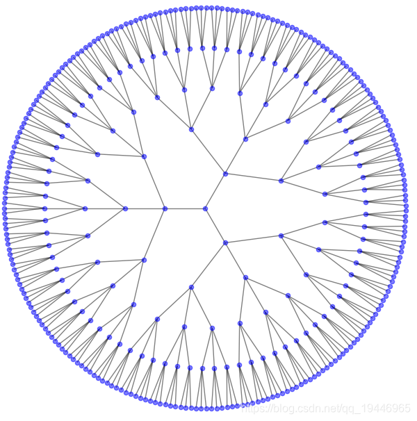
# 环形树状图
import os
import pydot
from networkx.drawing.nx_pydot import graphviz_layout

def set_prog(prog="dot"):

    path = r'C:\Program Files (x86)\Graphviz 2.28\bin'  # graphviz的bin目录
    prog = os.path.join(path, prog) + '.exe'
    return prog


G = nx.balanced_tree(3, 5)
pos = graphviz_layout(G, prog=set_prog("twopi"))
plt.figure(figsize=(8, 8))
nx.draw(G, pos, node_size=20, alpha=0.5, node_color="blue", with_labels=False)
plt.axis('equal')
plt.show()
2、权重图

G = nx.Graph()

G.add_edge('a', 'b', weight=0.6)
G.add_edge('a', 'c', weight=0.2)
G.add_edge('c', 'd', weight=0.1)
G.add_edge('c', 'e', weight=0.7)
G.add_edge('c', 'f', weight=0.9)
G.add_edge('a', 'd', weight=0.3)

elarge = [(u, v) for (u, v, d) in G.edges(data=True) if d['weight'] > 0.5]
esmall = [(u, v) for (u, v, d) in G.edges(data=True) if d['weight'] <= 0.5]

pos = nx.spring_layout(G)  # positions for all nodes

# nodes
nx.draw_networkx_nodes(G, pos, node_size=700)

# edges
nx.draw_networkx_edges(G, pos, edgelist=elarge, width=6)
nx.draw_networkx_edges(G, pos, edgelist=esmall, width=6, alpha=0.5, edge_color='b', style='dashed')

# labels-标签
# nx.draw_networkx_labels(G, pos, font_size=20, font_family='sans-serif')

plt.axis('off')
plt.show()
3、Giant Component
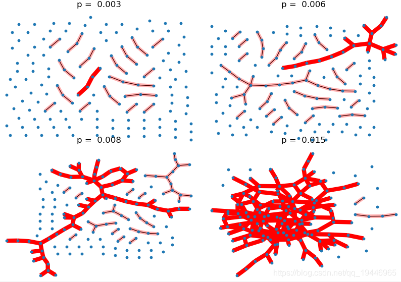
import pydot
from networkx.drawing.nx_pydot import graphviz_layout


def set_prog(prog="dot"):
    path = r'C:\Program Files (x86)\Graphviz 2.28\bin'  # graphviz的bin目录
    prog = os.path.join(path, prog) + '.exe'
    return prog


pvals = [0.003, 0.006, 0.008, 0.015]  # the range of p values should be close to the threshold

plt.subplots_adjust(left=0, right=1, bottom=0, top=0.95, wspace=0.01, hspace=0.01)
for i, p in enumerate(pvals):
    G = nx.binomial_graph(150, p)  # 150 nodes
    pos = graphviz_layout(G, prog=set_prog("neato"))
    plt.subplot(2, 2, i + 1)
    plt.title("p = %6.3f" % (p,))
    nx.draw(G, pos, with_labels=False, node_size=10)
    # 找出最大连通数的子图
    Gcc = sorted(nx.connected_component_subgraphs(G), key=len, reverse=True)
    G0 = Gcc[0]
    nx.draw_networkx_edges(G0, pos, with_labels=False, edge_color='r', width=6.0)
    # 画出其他连通数子图
    [nx.draw_networkx_edges(Gi, pos, with_labels=False, edge_color='r', alpha=0.3, width=5.0) for Gi in Gcc[1:] if
     len(Gi) > 1]
plt.show()
4、Random Geometric Graph 随机几何图
G = nx.random_geometric_graph(200, 0.125)
pos = nx.get_node_attributes(G, 'pos')  # position is stored as node attribute data for random_geometric_graph

# find node near center (0.5,0.5)
dmin = 1
ncenter = 0
for n in pos:
    x, y = pos[n]
    d = (x - 0.5) ** 2 + (y - 0.5) ** 2
    if d < dmin:
        ncenter = n
        dmin = d

# color by path length from node near center
p = dict(nx.single_source_shortest_path_length(G, ncenter))

plt.figure(figsize=(8, 8))
nx.draw_networkx_edges(G, pos, nodelist=[ncenter], alpha=0.4)
nx.draw_networkx_nodes(G, pos, nodelist=list(p.keys()), node_size=80,  node_color=list(p.values()), cmap=plt.cm.Reds_r)

plt.xlim(-0.05, 1.05)
plt.ylim(-0.05, 1.05)
plt.show()
5、节点颜色渐变
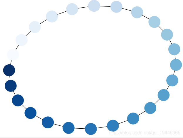
G = nx.cycle_graph(24)
pos = nx.spring_layout(G, iterations=200)
nx.draw(G, pos, node_color=range(24), node_size=800, cmap=plt.cm.Blues)
plt.show()
6、边颜色渐变
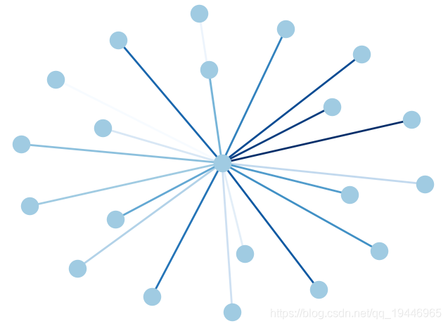
G = nx.star_graph(20)
pos = nx.spring_layout(G)  # 布局为中心放射状
colors = range(20)
nx.draw(G, pos, node_color='#A0CBE2', edge_color=colors, width=2, edge_cmap=plt.cm.Blues, with_labels=False)
plt.show()
7、Atlas
import os
import pydot
import random
from networkx.generators.atlas import graph_atlas_g
from networkx.drawing.nx_pydot import graphviz_layout
from networkx.algorithms.isomorphism.isomorph import graph_could_be_isomorphic as isomorphic


def set_prog(prog="dot"):
    path = r'C:\Program Files (x86)\Graphviz 2.28\bin'  # graphviz的bin目录
    prog = os.path.join(path, prog) + '.exe'
    return prog


def atlas6():
    """ Return the atlas of all connected graphs of 6 nodes or less.
        Attempt to check for isomorphisms and remove.
    """

    Atlas = graph_atlas_g()[0:208]  # 208
    # remove isolated nodes, only connected graphs are left
    U = nx.Graph()  # graph for union of all graphs in atlas
    for G in Atlas:
        for n in [n for n in G if G.degree(n) == 0]:
            G.remove_node(n)
        U = nx.disjoint_union(U, G)

    # iterator of graphs of all connected components
    C = (U.subgraph(c) for c in nx.connected_components(U))

    UU = nx.Graph()
    # do quick isomorphic-like check, not a true isomorphism checker
    nlist = []  # list of nonisomorphic graphs
    for G in C:
        # check against all nonisomorphic graphs so far
        if not iso(G, nlist):
            nlist.append(G)
            UU = nx.disjoint_union(UU, G)  # union the nonisomorphic graphs
    return UU


def iso(G1, glist):
    """Quick and dirty nonisomorphism checker used to check isomorphisms."""
    if any(isomorphic(G1, G2) for G2 in glist):
        return True
    return False


G = atlas6()
print("graph has %d nodes with %d edges" % (nx.number_of_nodes(G), nx.number_of_edges(G)))
print(nx.number_connected_components(G), "connected components")
plt.figure(1, figsize=(8, 8))
pos = graphviz_layout(G, prog=set_prog("neato"))
# color nodes the same in each connected subgraph
C = (G.subgraph(c) for c in nx.connected_components(G))
for g in C:
    c = [random.random()] * nx.number_of_nodes(g)  # random color...
    nx.draw(g, pos, node_size=40, node_color=c, vmin=0.0, vmax=1.0, with_labels=False)
plt.show()
8、Club

import networkx.algorithms.bipartite as bipartite

G = nx.davis_southern_women_graph()
women = G.graph['top']
clubs = G.graph['bottom']

print("Biadjacency matrix")
print(bipartite.biadjacency_matrix(G, women, clubs))

# project bipartite graph onto women nodes
W = bipartite.projected_graph(G, women)
print('')
print("#Friends, Member")
for w in women:
    print('%d %s' % (W.degree(w), w))

# project bipartite graph onto women nodes keeping number of co-occurence
# the degree computed is weighted and counts the total number of shared contacts
W = bipartite.weighted_projected_graph(G, women)
print('')
print("#Friend meetings, Member")
for w in women:
    print('%d %s' % (W.degree(w, weight='weight'), w))

nx.draw(G, node_color="red")
plt.show()
参考:
-
官方教程:
https://networkx.github.io/documentation/stable/_downloads/networkx_reference.pdf
-
官方网站:
https://networkx.github.io/documentation/latest/index.html
-
官方githu博客:
http://networkx.github.io/
-
https://blog.csdn.net/haoji007/article/details/103303507
-
https://blog.csdn.net/qq_30057549/article/details/104614857
-
https://www.cnblogs.com/shuodehaoa/p/8667045.html
-
https://blog.csdn.net/darren2015zdc/article/details/75012508
-
https://blog.csdn.net/ciyiquan5963/article/details/78489595
-
http://www.downza.cn/soft/284938.html
-
https://blog.csdn.net/weixin_41864878/article/details/81095885