导入计算库
import pandas as pd
import numpy as np
import matplotlib.pyplot as plt
import seaborn as sns
plt.style.use("fivethirtyeight")
plt.rcParams["font.sans-serif"] = ["Microsoft YaHei"]
plt.rcParams["axes.unicode_minus"] = False
from sklearn.preprocessing import OneHotEncoder

import statsmodels.api as sm
from statsmodels.graphics.tsaplots import plot_acf,plot_pacf
from pandas.tseries.offsets import DateOffset


from statsmodels.tsa.arima.model import ARIMA

import warnings
warnings.filterwarnings("ignore")
导入数据
path_train = "../preocess_data/train_data_o.csv"
path_test = "../data/test_data.csv"
data  = pd.read_csv(path_train)
data_test = pd.read_csv(path_test)
data["运营日期"] = pd.to_datetime(data["运营日期"] )
data_test["运营日期"] = pd.to_datetime(data_test["日期"])
data.drop(["行ID","日期"],axis=1,inplace=True)
data_test.drop(["行ID","日期"],axis=1,inplace=True)
折扣编码
enc = OneHotEncoder(drop="if_binary")
enc.fit(data["折扣"].values.reshape(-1,1))
enc.transform(data["折扣"].values.reshape(-1,1)).toarray()
enc.transform(data_test["折扣"].values.reshape(-1,1)).toarray()
array([[0.],
       [0.],
       [0.],
       ...,
       [1.],
       [0.],
       [0.]])
data["折扣"] = enc.transform(data["折扣"].values.reshape(-1,1)).toarray()
data_test["折扣"]  = enc.transform(data_test["折扣"].values.reshape(-1,1)).toarray()
日期衍生
def time_derivation(t,col="运营日期"):
    t["year"] = t[col].dt.year
    t["month"] = t[col].dt.month
    t["day"] = t[col].dt.day
    t["quarter"] = t[col].dt.quarter
    t["weekofyear"] = t[col].dt.weekofyear
    t["dayofweek"] = t[col].dt.dayofweek+1
    t["weekend"] = (t["dayofweek"]>5).astype(int)
    return t

data_train  = time_derivation(data)
data_test_  = time_derivation(data_test)
对每家店进行探索
对第一家尝试
# 训练集合
data_train_1 = data_train[data_train["商店ID"] ==1]
# 测试集合
data_test_1 = data_test_[data_test_["商店ID"] ==1]
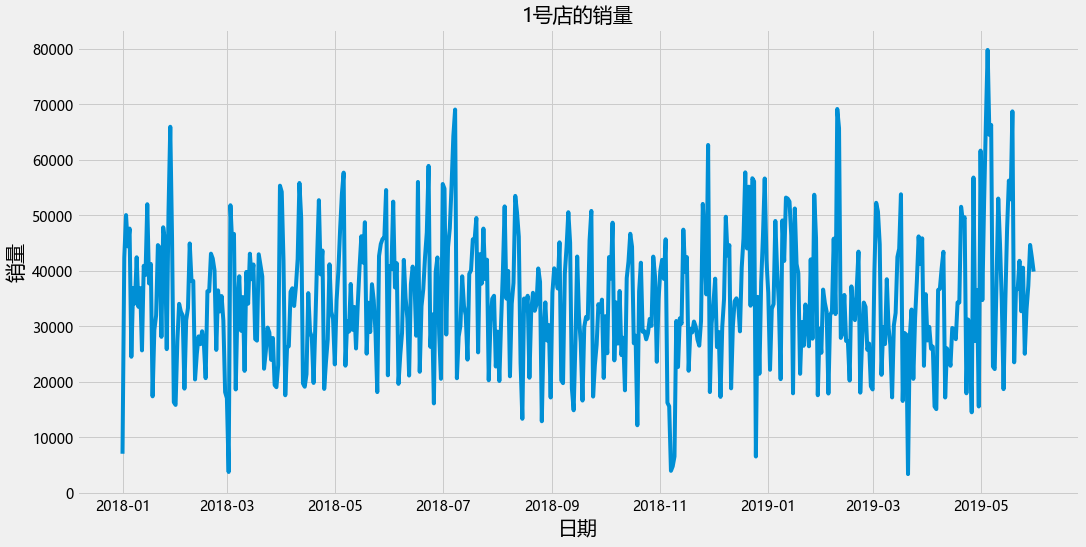
plt.figure(figsize=(16,8))
plt.plot(data_train_1["运营日期"],data_train_1["销量"])
plt.xlabel("日期",fontsize= 20)
plt.ylabel("销量",fontsize= 20)
plt.title("1号店的销量",fontsize=20)
Text(0.5, 1.0, '1号店的销量')
开始尝试
data_train_1.head()
| 商店ID | 商店类型 | 位置 | 地区 | 节假日 | 折扣 | 销量 | 运营日期 | year | month | day | quarter | weekofyear | dayofweek | weekend | |
|---|---|---|---|---|---|---|---|---|---|---|---|---|---|---|---|
| 0 | 1 | S1 | L3 | R1 | 1 | 1.0 | 7011.84 | 2018-01-01 | 2018 | 1 | 1 | 1 | 1 | 1 | 0 |
| 607 | 1 | S1 | L3 | R1 | 0 | 1.0 | 42369.00 | 2018-01-02 | 2018 | 1 | 2 | 1 | 1 | 2 | 0 |
| 1046 | 1 | S1 | L3 | R1 | 0 | 1.0 | 50037.00 | 2018-01-03 | 2018 | 1 | 3 | 1 | 1 | 3 | 0 |
| 1207 | 1 | S1 | L3 | R1 | 0 | 1.0 | 44397.00 | 2018-01-04 | 2018 | 1 | 4 | 1 | 1 | 4 | 0 |
| 1752 | 1 | S1 | L3 | R1 | 0 | 1.0 | 47604.00 | 2018-01-05 | 2018 | 1 | 5 | 1 | 1 | 5 | 0 |
复制获得数据
data_train__1 = data_train_1.copy()
data_test__1 = data_test_1.copy()
删除不变的属性
data_train__1.drop(["商店类型","商店ID","位置","地区","运营日期"],axis=1,inplace=True)
data_test__1.drop(["商店类型","商店ID","位置","地区","运营日期"],axis=1,inplace=True)
在这里留下一个思考的点, 其实节假日的附近几天的属性也会对预测结果产生一定影响。
data_train__1.shape
(516, 10)
data_train__1
| 节假日 | 折扣 | 销量 | year | month | day | quarter | weekofyear | dayofweek | weekend | |
|---|---|---|---|---|---|---|---|---|---|---|
| 0 | 1 | 1.0 | 7011.84 | 2018 | 1 | 1 | 1 | 1 | 1 | 0 |
| 607 | 0 | 1.0 | 42369.00 | 2018 | 1 | 2 | 1 | 1 | 2 | 0 |
| 1046 | 0 | 1.0 | 50037.00 | 2018 | 1 | 3 | 1 | 1 | 3 | 0 |
| 1207 | 0 | 1.0 | 44397.00 | 2018 | 1 | 4 | 1 | 1 | 4 | 0 |
| 1752 | 0 | 1.0 | 47604.00 | 2018 | 1 | 5 | 1 | 1 | 5 | 0 |
| … | … | … | … | … | … | … | … | … | … | … |
| 186569 | 0 | 1.0 | 33075.00 | 2019 | 5 | 27 | 2 | 22 | 1 | 0 |
| 187165 | 0 | 1.0 | 37317.00 | 2019 | 5 | 28 | 2 | 22 | 2 | 0 |
| 187391 | 0 | 1.0 | 44652.00 | 2019 | 5 | 29 | 2 | 22 | 3 | 0 |
| 187962 | 0 | 1.0 | 42387.00 | 2019 | 5 | 30 | 2 | 22 | 4 | 0 |
| 188113 | 1 | 1.0 | 39843.78 | 2019 | 5 | 31 | 2 | 22 | 5 | 0 |
516 rows × 10 columns
data_train__1["diff_1"] = data_train__1["销量"].diff(10)
data_train__1 = data_train__1.dropna()

# data_test__1["diff_1"] = data_test__1["销量"].diff(1)
# data_test__1 = data_test__1.dropna()
将数据集变为有监督数据集
def series_to_supervisied_(data,step_in,step_out,dropnan = True):
    """
    :param data: 观测的序列,类型为列表或者二维的numpy数组
    :param step_in: 作为输入滞后观测数量(x)
    :param step_out: 作为输出的观测值数量(y)
    :param  dropnan: 是否具有Nan的行,默认为True
    return 监督学习的重组得到的dataframe列
    """
    n_vars = 1 if type(data) is list else data.shape[1]
    df = data
    cols = []
    names = []
    # 输入序列[(t-n),(t-n+1),(t-n+2)..(t-1)]
    for i in range(step_in,0,-1):
        cols.append(df.shift(i))
        names+=[f"{name}-({i})step" for name in df.columns]
    # 输出序列[t,(t+1),(t+2)...(t+n)]
    for i in range(0,step_out):
        cols.append(df.shift(-i))
        if i ==0:
            names+=[f"{name}+(0)step" for name in df.columns]
        else:
            names+=[f"{name}+({i})step" for name in df.columns]

    df_re = pd.concat(cols,axis=1)
    df_re.columns = names
    if dropnan:
        df_re.dropna(inplace=True)

    return df_re
data_step = series_to_supervisied_(data_train__1,step_in= 10,step_out=2,dropnan = True)
data_step
| 节假日-(10)step | 折扣-(10)step | 销量-(10)step | year-(10)step | month-(10)step | day-(10)step | quarter-(10)step | weekofyear-(10)step | dayofweek-(10)step | weekend-(10)step | … | 折扣+(1)step | 销量+(1)step | year+(1)step | month+(1)step | day+(1)step | quarter+(1)step | weekofyear+(1)step | dayofweek+(1)step | weekend+(1)step | diff_1+(1)step | |
|---|---|---|---|---|---|---|---|---|---|---|---|---|---|---|---|---|---|---|---|---|---|
| 7658 | 0.0 | 0.0 | 36873.00 | 2018.0 | 1.0 | 11.0 | 1.0 | 2.0 | 4.0 | 0.0 | … | 0.0 | 44178.75 | 2018.0 | 1.0 | 22.0 | 1.0 | 4.0 | 1.0 | 0.0 | 18534.75 |
| 7791 | 0.0 | 0.0 | 25644.00 | 2018.0 | 1.0 | 12.0 | 1.0 | 2.0 | 5.0 | 0.0 | … | 0.0 | 28086.00 | 2018.0 | 1.0 | 23.0 | 1.0 | 4.0 | 2.0 | 0.0 | -12804.00 |
| 8337 | 0.0 | 1.0 | 40890.00 | 2018.0 | 1.0 | 13.0 | 1.0 | 2.0 | 6.0 | 1.0 | … | 0.0 | 47835.00 | 2018.0 | 1.0 | 24.0 | 1.0 | 4.0 | 3.0 | 0.0 | 8580.60 |
| 8610 | 1.0 | 1.0 | 39254.40 | 2018.0 | 1.0 | 14.0 | 1.0 | 2.0 | 7.0 | 1.0 | … | 1.0 | 45384.00 | 2018.0 | 1.0 | 25.0 | 1.0 | 4.0 | 4.0 | 0.0 | -6609.00 |
| 8821 | 0.0 | 1.0 | 51993.00 | 2018.0 | 1.0 | 15.0 | 1.0 | 3.0 | 1.0 | 0.0 | … | 1.0 | 25868.88 | 2018.0 | 1.0 | 26.0 | 1.0 | 4.0 | 5.0 | 0.0 | -11847.12 |
| … | … | … | … | … | … | … | … | … | … | … | … | … | … | … | … | … | … | … | … | … | … |
| 186152 | 0.0 | 1.0 | 47619.00 | 2019.0 | 5.0 | 16.0 | 2.0 | 20.0 | 4.0 | 0.0 | … | 1.0 | 33075.00 | 2019.0 | 5.0 | 27.0 | 2.0 | 22.0 | 1.0 | 0.0 | -23178.00 |
| 186569 | 0.0 | 1.0 | 56253.00 | 2019.0 | 5.0 | 17.0 | 2.0 | 20.0 | 5.0 | 0.0 | … | 1.0 | 37317.00 | 2019.0 | 5.0 | 28.0 | 2.0 | 22.0 | 2.0 | 0.0 | -15560.82 |
| 187165 | 1.0 | 1.0 | 52877.82 | 2019.0 | 5.0 | 18.0 | 2.0 | 20.0 | 6.0 | 1.0 | … | 1.0 | 44652.00 | 2019.0 | 5.0 | 29.0 | 2.0 | 22.0 | 3.0 | 0.0 | -24081.00 |
| 187391 | 0.0 | 1.0 | 68733.00 | 2019.0 | 5.0 | 19.0 | 2.0 | 20.0 | 7.0 | 1.0 | … | 1.0 | 42387.00 | 2019.0 | 5.0 | 30.0 | 2.0 | 22.0 | 4.0 | 0.0 | 18891.00 |
| 187962 | 0.0 | 0.0 | 23496.00 | 2019.0 | 5.0 | 20.0 | 2.0 | 21.0 | 1.0 | 0.0 | … | 1.0 | 39843.78 | 2019.0 | 5.0 | 31.0 | 2.0 | 22.0 | 5.0 | 0.0 | 3231.78 |
495 rows × 132 columns
list(data_step.columns)[-11:]
['节假日+(1)step',
 '折扣+(1)step',
 '销量+(1)step',
 'year+(1)step',
 'month+(1)step',
 'day+(1)step',
 'quarter+(1)step',
 'weekofyear+(1)step',
 'dayofweek+(1)step',
 'weekend+(1)step',
 'diff_1+(1)step']
y_columns = "销量+(1)step"
y = data_step[y_columns]
x = data_step[list(data_step.columns)[:-11]]
data_ = pd.concat([x,y],axis=1)
data_
| 节假日-(10)step | 折扣-(10)step | 销量-(10)step | year-(10)step | month-(10)step | day-(10)step | quarter-(10)step | weekofyear-(10)step | dayofweek-(10)step | weekend-(10)step | … | 销量+(0)step | year+(0)step | month+(0)step | day+(0)step | quarter+(0)step | weekofyear+(0)step | dayofweek+(0)step | weekend+(0)step | diff_1+(0)step | 销量+(1)step | |
|---|---|---|---|---|---|---|---|---|---|---|---|---|---|---|---|---|---|---|---|---|---|
| 7658 | 0.0 | 0.0 | 36873.00 | 2018.0 | 1.0 | 11.0 | 1.0 | 2.0 | 4.0 | 0.0 | … | 44625.00 | 2018 | 1 | 21 | 1 | 3 | 7 | 1 | 7752.00 | 44178.75 |
| 7791 | 0.0 | 0.0 | 25644.00 | 2018.0 | 1.0 | 12.0 | 1.0 | 2.0 | 5.0 | 0.0 | … | 44178.75 | 2018 | 1 | 22 | 1 | 4 | 1 | 0 | 18534.75 | 28086.00 |
| 8337 | 0.0 | 1.0 | 40890.00 | 2018.0 | 1.0 | 13.0 | 1.0 | 2.0 | 6.0 | 1.0 | … | 28086.00 | 2018 | 1 | 23 | 1 | 4 | 2 | 0 | -12804.00 | 47835.00 |
| 8610 | 1.0 | 1.0 | 39254.40 | 2018.0 | 1.0 | 14.0 | 1.0 | 2.0 | 7.0 | 1.0 | … | 47835.00 | 2018 | 1 | 24 | 1 | 4 | 3 | 0 | 8580.60 | 45384.00 |
| 8821 | 0.0 | 1.0 | 51993.00 | 2018.0 | 1.0 | 15.0 | 1.0 | 3.0 | 1.0 | 0.0 | … | 45384.00 | 2018 | 1 | 25 | 1 | 4 | 4 | 0 | -6609.00 | 25868.88 |
| … | … | … | … | … | … | … | … | … | … | … | … | … | … | … | … | … | … | … | … | … | … |
| 186152 | 0.0 | 1.0 | 47619.00 | 2019.0 | 5.0 | 16.0 | 2.0 | 20.0 | 4.0 | 0.0 | … | 25035.00 | 2019 | 5 | 26 | 2 | 21 | 7 | 1 | -22584.00 | 33075.00 |
| 186569 | 0.0 | 1.0 | 56253.00 | 2019.0 | 5.0 | 17.0 | 2.0 | 20.0 | 5.0 | 0.0 | … | 33075.00 | 2019 | 5 | 27 | 2 | 22 | 1 | 0 | -23178.00 | 37317.00 |
| 187165 | 1.0 | 1.0 | 52877.82 | 2019.0 | 5.0 | 18.0 | 2.0 | 20.0 | 6.0 | 1.0 | … | 37317.00 | 2019 | 5 | 28 | 2 | 22 | 2 | 0 | -15560.82 | 44652.00 |
| 187391 | 0.0 | 1.0 | 68733.00 | 2019.0 | 5.0 | 19.0 | 2.0 | 20.0 | 7.0 | 1.0 | … | 44652.00 | 2019 | 5 | 29 | 2 | 22 | 3 | 0 | -24081.00 | 42387.00 |
| 187962 | 0.0 | 0.0 | 23496.00 | 2019.0 | 5.0 | 20.0 | 2.0 | 21.0 | 1.0 | 0.0 | … | 42387.00 | 2019 | 5 | 30 | 2 | 22 | 4 | 0 | 18891.00 | 39843.78 |
495 rows × 122 columns
划分训练集测试集
lens = -1
from sklearn.model_selection import train_test_split
from sklearn.utils import shuffle
data_train_,data_test_ = train_test_split(data_,test_size=0.2,shuffle=False)
data_train_  = shuffle(data_train_,random_state=1412)
xtrain,ytrain = data_train_.iloc[:,:lens],data_train_.iloc[:,lens]
xtest,ytest = data_test_.iloc[:,:lens],data_test_.iloc[:,lens]
归一化
from sklearn.preprocessing import MinMaxScaler
scaler = MinMaxScaler()
scaler.fit(ytrain.values.reshape(-1,1))
y_train = scaler.transform(ytrain.values.reshape(-1,1))
y_test = scaler.transform(ytest.values.reshape(-1,1))
随机森林
from sklearn.ensemble import RandomForestRegressor
rf_clf = RandomForestRegressor(max_depth=12,
                               min_impurity_decrease=0.0,
                               n_estimators= 300)
rf_clf.fit(xtrain,ytrain)
rf_clf.score(xtest,ytest)
0.43699715354836455
from sklearn.metrics import mean_squared_error
mean_squared_error(ytest,rf_clf.predict(xtest))**0.5
10330.02670862774
mean_squared_error(ytrain,rf_clf.predict(xtrain))**0.5
3440.408502696517
def symmetric_mean_absolute_percentage_error(y_true, y_pred):
    y_true, y_pred = np.array(y_true), np.array(y_pred)
    return np.sum(np.abs(y_true - y_pred) * 2) / np.sum(np.abs(y_true) + np.abs(y_pred))

def prophet_smape(y_true, y_pred):
    smape_val = symmetric_mean_absolute_percentage_error(y_true, y_pred)
    return 'SMAPE', smape_val, False
prophet_smape(ytrain,rf_clf.predict(xtrain))
('SMAPE', 0.07417421103653893, False)
prophet_smape(ytest,rf_clf.predict(xtest))
xgboost
from xgboost import XGBRegressor
xgb_clf = XGBRegressor(max_depth=12,
                               n_estimators=500)
xgb_clf.fit(xtrain,ytrain)
xgb_clf.score(xtest,ytest)
0.40055294233563
mean_squared_error(ytest,xgb_clf.predict(xtest))**0.5
10659.125252942618
mean_squared_error(ytrain,xgb_clf.predict(xtrain))**0.5
0.0036928046625203763
prophet_smape(ytest,xgb_clf.predict(xtest))
('SMAPE', 0.22077657322671448, False)
prophet_smape(ytrain,xgb_clf.predict(xtrain))
('SMAPE', 7.480844639369475e-08, False)
用一下贝叶斯优化看一下,是不是历史时间步长的问题?
from hyperopt import hp,fmin,tpe,Trials,partial
from hyperopt.early_stop import no_progress_loss


# 定义目标函数:
def hpyeropt_objective(params):

    data_step = series_to_supervisied_(data_train__1,step_in = int(params["time_step"]),step_out=2,dropnan = True)

    y_columns = "销量+(0)step"
    y = data_step[y_columns]
    x = data_step[list(data_step.columns)[:-20]]
    data_ = pd.concat([x,y],axis=1)

    from sklearn.model_selection import train_test_split
    from sklearn.utils import shuffle
    data_train,data_test = train_test_split(data_,test_size=0.2,shuffle=False)
    data_train  = shuffle(data_train,random_state=1412)
    xtrain,ytrain = data_train.iloc[:,:-20],data_train.iloc[:,-1]
    xtest,ytest = data_test.iloc[:,:-20],data_test.iloc[:,-1]

    # 归一化
    from sklearn.preprocessing import MinMaxScaler
    scaler = MinMaxScaler()
    scaler.fit(ytrain.values.reshape(-1,1))
    ytrain = scaler.transform(ytrain.values.reshape(-1,1))
    ytest = scaler.transform(ytest.values.reshape(-1,1))


    clf = RandomForestRegressor(n_estimators=int(params["n_estimators"]),
                                max_depth=int(params["max_depth"]),
#                                max_features=int(min(params["max_features"],len(xtrain.columns))),
                               min_impurity_decrease=params["min_impurity_decrease"],
                               random_state=1412,
                               verbose=False,
                               n_jobs=-1
                               ).fit(xtrain,ytrain)

    scores = clf.score(xtest,ytest)
    return -scores


#定义参数空间
params_grid = {"n_estimators":hp.quniform("n_estimators",10,1000,20),
                   "max_depth":hp.quniform("max_depth",5,25,1),
#                    "max_features":hp.quniform("max_features",10,10000,1),
                   "min_impurity_decrease":hp.quniform("min_impurity_decrease",0,5,1),


               "time_step":hp.quniform("time_step",10,200,5)
              }

#定义迭代
def param_hyperopt(max_evals = 100):
    trials = Trials()
    early_stop_fn =no_progress_loss(50)
    params_best = fmin(hpyeropt_objective,
                      space=params_grid,
                       algo=tpe.suggest,
                       max_evals=max_evals,
                       verbose=True,
                       trials=trials,
                       early_stop_fn=early_stop_fn
                      )
    print("\n","\n","best params:",params_best,"\n")
    return params_best,trials
params_best,trials = param_hyperopt(max_evals = 300)
34%|███████████████ | 103/300 [02:59<05:43, 1.75s/trial, best loss: -0.48958559215129405]
best params: {‘max_depth’: 9.0, ‘min_impurity_decrease’: 0.0, ‘n_estimators’: 660.0, ‘time_step’: 10.0}
目前来讲的话,效果都不是很好,那么接下来从时间角度来想的话,在每个时间窗内进行差分以及其他的特征衍生,尽量的提取一些其他的特征! 至此先考虑下另外一个方案。
data_train__1["销量"].diff()-data_train__1["销量"].diff()
| 节假日 | 折扣 | 销量 | year | month | day | quarter | weekofyear | dayofweek | weekend | |
|---|---|---|---|---|---|---|---|---|---|---|
| 0 | 1.0 | 0.0 | -35357.16 | 0.0 | 0.0 | -1.0 | 0.0 | 0.0 | -1.0 | 0.0 |
| 607 | 0.0 | 0.0 | -7668.00 | 0.0 | 0.0 | -1.0 | 0.0 | 0.0 | -1.0 | 0.0 |
| 1046 | 0.0 | 0.0 | 5640.00 | 0.0 | 0.0 | -1.0 | 0.0 | 0.0 | -1.0 | 0.0 |
| 1207 | 0.0 | 0.0 | -3207.00 | 0.0 | 0.0 | -1.0 | 0.0 | 0.0 | -1.0 | 0.0 |
| 1752 | 0.0 | 1.0 | 23109.00 | 0.0 | 0.0 | -1.0 | 0.0 | 0.0 | -1.0 | -1.0 |
| … | … | … | … | … | … | … | … | … | … | … |
| 186569 | 0.0 | 0.0 | -4242.00 | 0.0 | 0.0 | -1.0 | 0.0 | 0.0 | -1.0 | 0.0 |
| 187165 | 0.0 | 0.0 | -7335.00 | 0.0 | 0.0 | -1.0 | 0.0 | 0.0 | -1.0 | 0.0 |
| 187391 | 0.0 | 0.0 | 2265.00 | 0.0 | 0.0 | -1.0 | 0.0 | 0.0 | -1.0 | 0.0 |
| 187962 | -1.0 | 0.0 | 2543.22 | 0.0 | 0.0 | -1.0 | 0.0 | 0.0 | -1.0 | 0.0 |
| 188113 | NaN | NaN | NaN | NaN | NaN | NaN | NaN | NaN | NaN | NaN |
516 rows × 10 columns
版权声明:本文为qq_39215918原创文章,遵循 CC 4.0 BY-SA 版权协议,转载请附上原文出处链接和本声明。