roc.wfns <- roc(aSAH$outcome, aSAH$wfns)
## Setting levels: control = Good, case = Poor
## Setting direction: controls < cases

roc.ndka <- roc(aSAH$outcome, aSAH$ndka)
## Setting levels: control = Good, case = Poor
## Setting direction: controls < cases

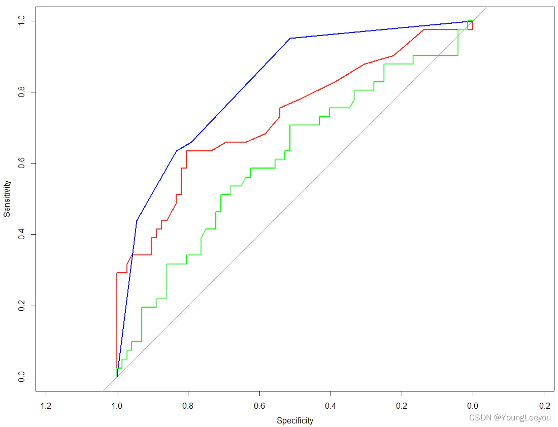
# Add a second ROC curve to the previous plot:
plot(roc.s100b, col="red")
plot(roc.wfns, col="blue", add=TRUE)
plot(roc.ndka, col="green", add=TRUE)

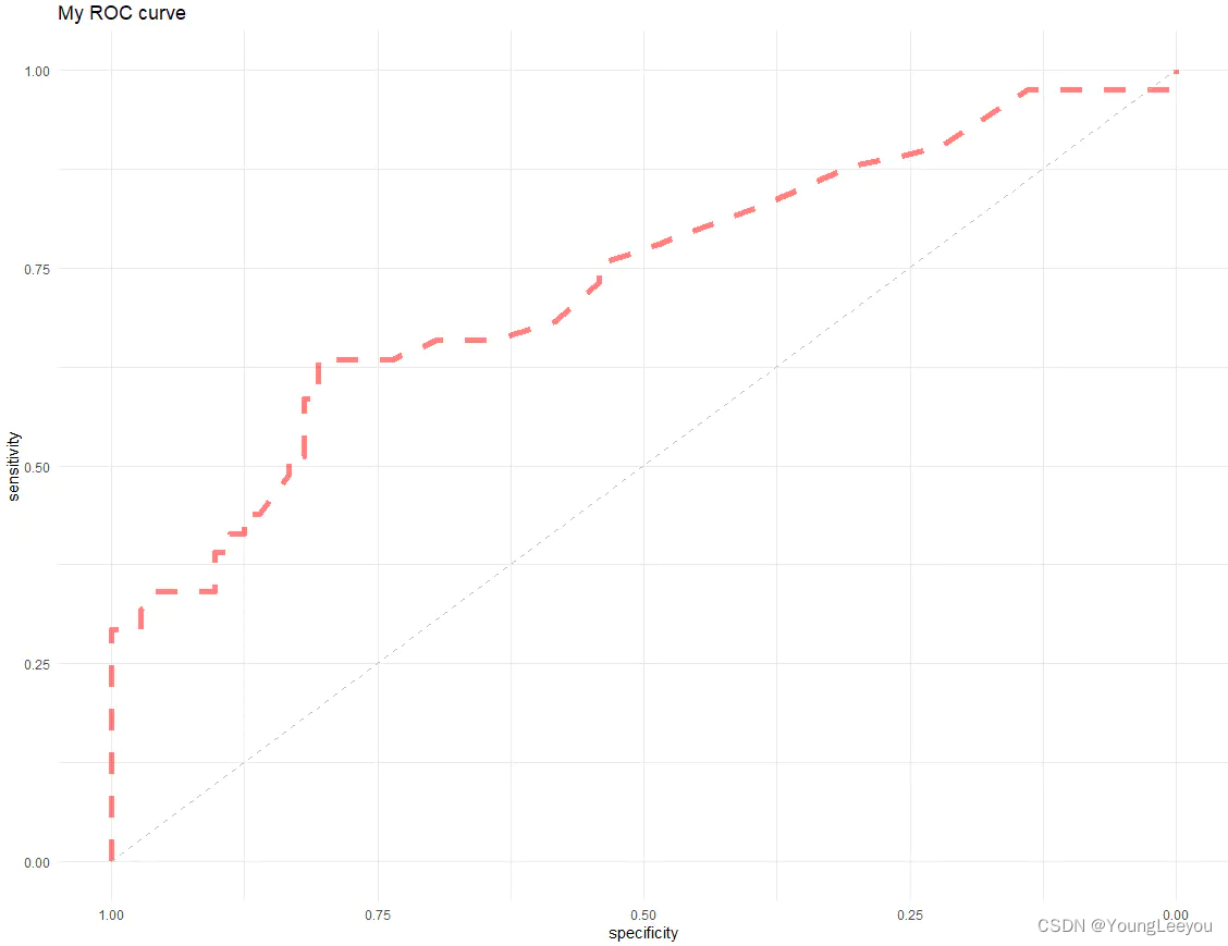
使用ggcor()函数绘制基于ggplot2的ROC曲线

ggroc(roc.s100b, 
      alpha = 0.5, colour = "red", 
      linetype = 2, size = 2) +
  theme_minimal() + 
  ggtitle("My ROC curve") + 
  geom_segment(aes(x = 1, xend = 0, y = 0, yend = 1), 
               color="grey", linetype="dashed")

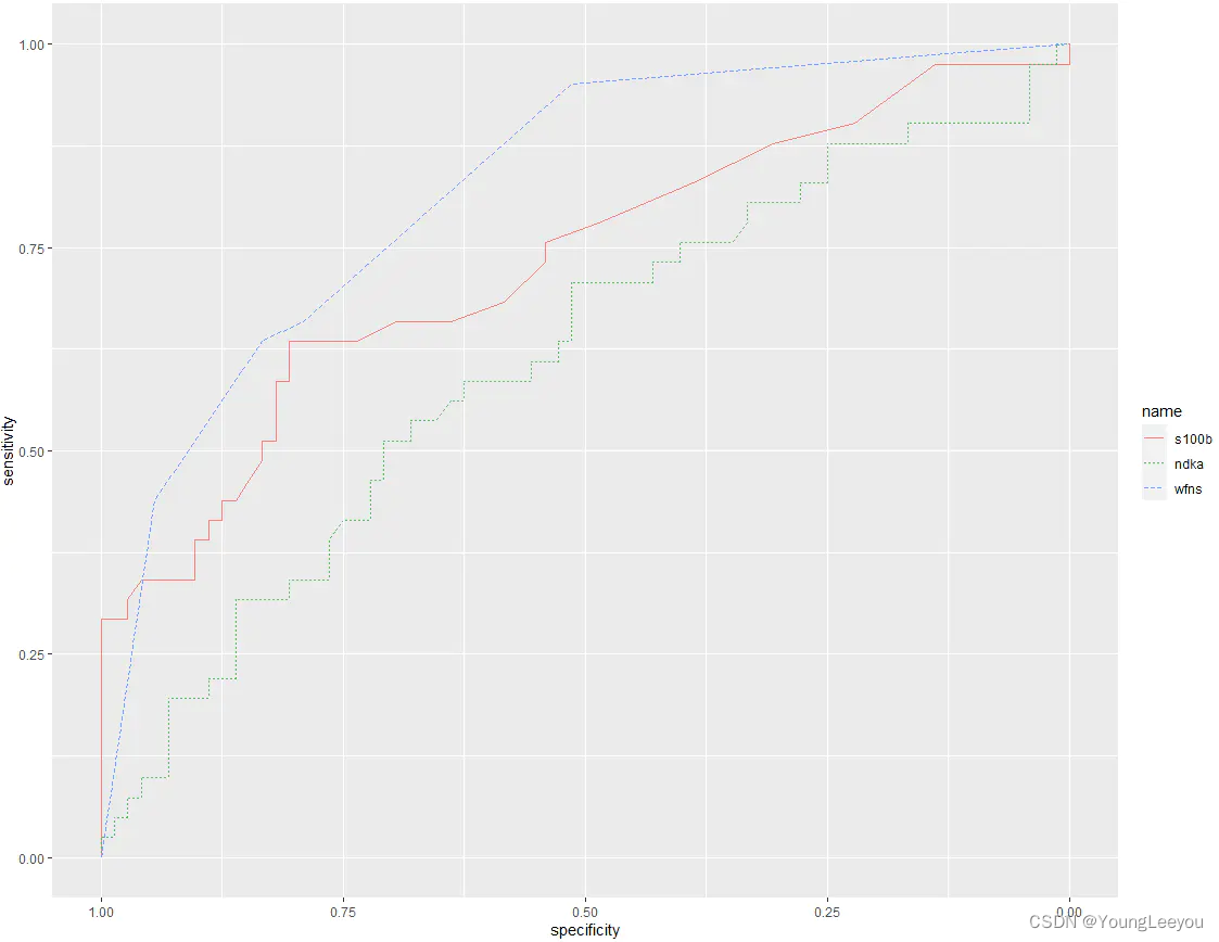
绘制多条ROC曲线

Multiple curves:

ggroc(list(s100b=roc.s100b, wfns=roc.wfns, ndka=roc.ndka))

# This is equivalent to using roc.formula:
roc.list <- roc(outcome ~ s100b + ndka + wfns, data = aSAH)
## Setting levels: control = Good, case = Poor
## Setting direction: controls < cases
## Setting levels: control = Good, case = Poor
## Setting direction: controls < cases
## Setting levels: control = Good, case = Poor
## Setting direction: controls < cases

g.list <- ggroc(roc.list, aes=c("linetype", "color"))
g.list

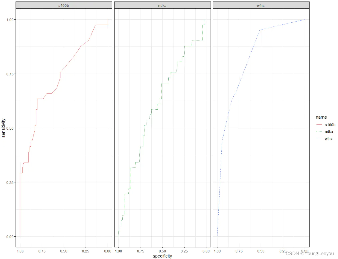
分面展示

# OR faceting
g.list + facet_grid(.~name) + 
  theme_bw() 

使用survivalROC包绘制时间依赖的ROC曲线

# 安装并加载所需的R包
#install.packages("survivalROC")
library(survivalROC)

# 查看内置数据集
data(mayo)
head(mayo)
##   time censor mayoscore5 mayoscore4
## 1   41      1  11.251850  10.629450
## 2  179      1  10.136070  10.185220
## 3  334      1  10.095740   9.422995
## 4  400      1  10.189150   9.567799
## 5  130      1   9.770148   9.039419
## 6  223      1   9.226429   9.033388

# 计算数据的行数
nobs <- NROW(mayo)
nobs
## [1] 312

# 自定义阈值
cutoff <- 365

# 使用MAYOSCORE 4作为marker, 并用NNE（Nearest Neighbor Estimation）法计算ROC值
Mayo4.1 = survivalROC(Stime=mayo$time,  
                      status=mayo$censor,      
                      marker = mayo$mayoscore4,     
                      predict.time = cutoff,
                      span = 0.25*nobs^(-0.20) )
Mayo4.1

# 绘制ROC曲线
plot(Mayo4.1$FP, Mayo4.1$TP, type="l", 
     xlim=c(0,1), ylim=c(0,1), col="red",  
     xlab=paste( "FP", "\n", "AUC = ",round(Mayo4.1$AUC,3)), 
     ylab="TP",main="Mayoscore 4, Method = NNE \n  Year = 1")
# 添加对角线
abline(0,1)

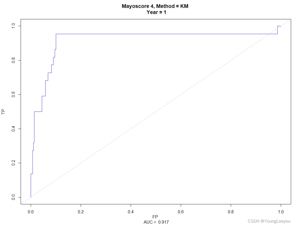
使用KM（Kaplan-Meier）法计算ROC值

## MAYOSCORE 4, METHOD = KM
Mayo4.2= survivalROC(Stime=mayo$time,  
                     status=mayo$censor,      
                     marker = mayo$mayoscore4,     
                     predict.time =  cutoff, method="KM")
Mayo4.2

plot(Mayo4.2$FP, Mayo4.2$TP, type="l", 
     xlim=c(0,1), ylim=c(0,1), col="blue",
     xlab=paste( "FP", "\n", "AUC = ",round(Mayo4.2$AUC,3)), 
     ylab="TP",main="Mayoscore 4, Method = KM \n Year = 1")
abline(0,1,lty=2,col="gray")

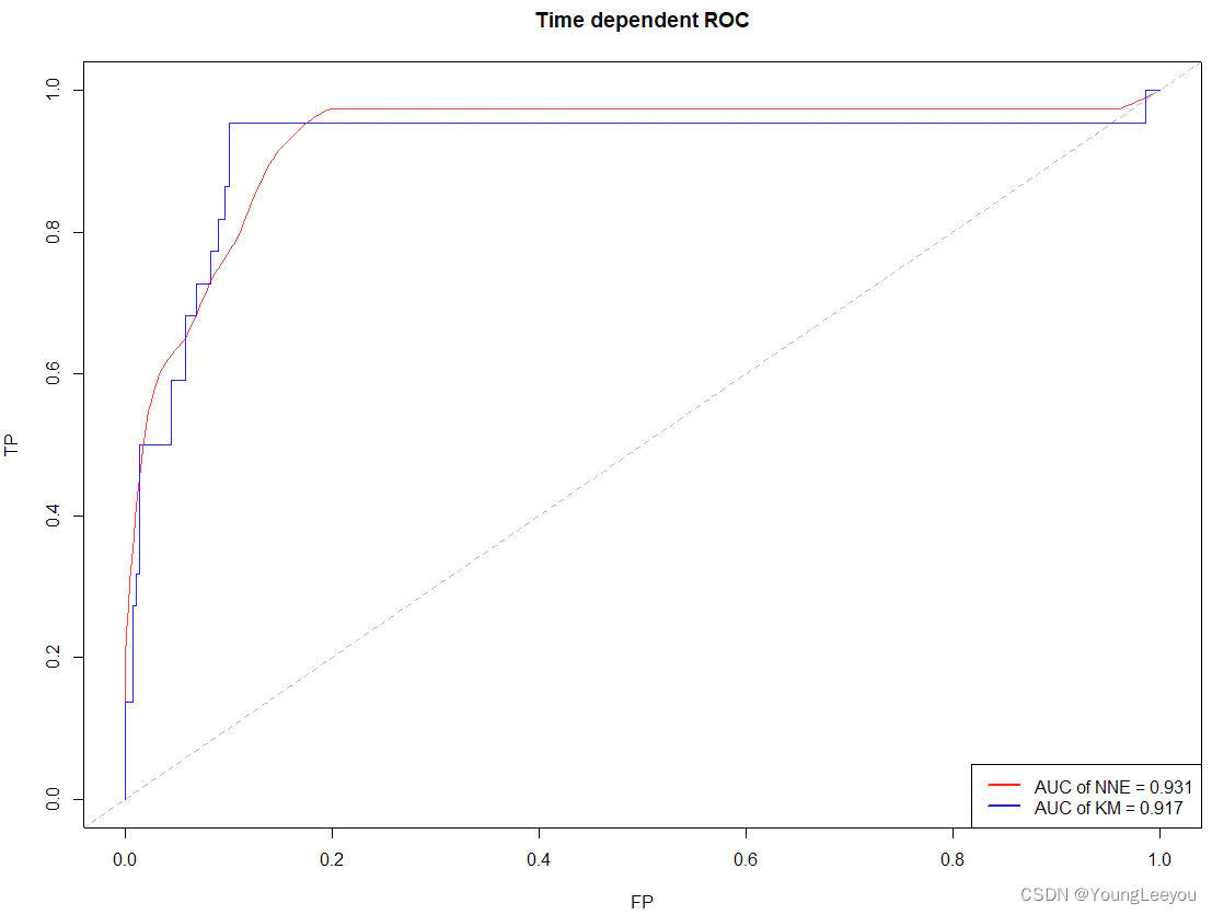
# 将两种方法的结果绘制到同一个图里
## 绘制NNE法计算的ROC曲线
plot(Mayo4.1$FP, Mayo4.1$TP,
     type="l",col="red",
     xlim=c(0,1), ylim=c(0,1),   
     xlab="FP", 
     ylab="TP",
     main="Time dependent ROC")
# 添加对角线
abline(0,1,col="gray",lty=2)

## 添加KM法计算的ROC曲线
lines(Mayo4.2$FP, Mayo4.2$TP, 
      type="l",col="blue",
      xlim=c(0,1), ylim=c(0,1))
# 添加图例
legend("bottomright",legend = c(paste("AUC of NNE =",round(Mayo4.1$AUC,3)),
                          paste("AUC of KM =",round(Mayo4.2$AUC,3))),
       col=c("red","blue"),
       lty= 1 ,lwd= 2)