第十一章 方差分析表(analysis of variance table)ANOVA TABLE

  • Post author:
  • Post category:其他


11.1 方差分析表概念

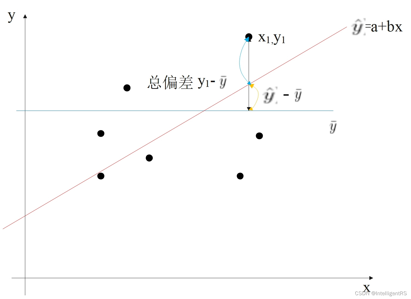
回归平方和:SSR(Sum of Squares for regression) = ESS (explained sum of squares)

残差平方和:SSE(Sum of Squares for Error) = RSS (residual sum of squares)

总离差平方和:SST(Sum of Squares for total) = TSS(total sum of squares)


SSE+SSR=SST RSS+ESS=TSS

TSS = (Y_1-\overline{Y})^2+(Y_2-\overline{Y})^2+(Y_3-\overline{Y})^2+......

RSS = (\hat{Y_1}-\overline{Y})^2 + (\hat{Y_2}-\overline{Y})^2+(\hat{Y_3}-\overline{Y})^2+......

SSE = (y_1-\hat{y})^2+(y_2-\hat{y})^2+ (y_3-\hat{y})^2+......=(e_1)^2+(e_2)^2+(e_3)^2+......

TSS = SSE + RSS

R^2
(决定系数 Coefficient of Determination):

(1)R^2 = \frac{RSS(Explained\;Variation)}{TSS(Total\;Variation)} = 1-\frac{SSE(Unexplained\;Variation)}{TSS(Total\;Variation)}
(2)0\leq R^2\leq 1\;R^2
越接近于1,解释力度越大

(3)R^2=r^2

SEE(Standard Error of Estimate):

Actual Y – Estimated Y

SEE = \sqrt{\frac{SSE}{n-2}}=\sqrt{MSE}

SEE = \sqrt{\frac{(e_1-\bar{e})^2+(e_2-\bar{e})^2+(e_3-\bar{e})^2+......}{n-k-1}}

SSE = (y_1-\hat{y})^2+(y_2-\hat{y})^2+(y_3-\hat{y})^2+......=(e_1)^2+(e_2)^2+(e_3)^2+......

而此时,
\bar{e}
为一个垃圾桶,均值为0。

11.2 检验

11.2.1 T检验

(1)点估计(point estimation)
C=100*H+88\;--->H->\hat{b_1}\;88->\hat{b_0}

(2)置信区间(Confident Interval)
b_1\;95%\;b_1(\hat{b_1}\pm 1.96S_{\hat{b_1}})

S_{\hat{b_1}
如果增大,SEE相应上升,因为本质上SEE是描述数据的波动性(variability of data)


检验方法:假设检验

(1)

H_0:b_1=0

H_a:b_1\neq0

(2)

t=\frac{\hat{b_1}-0}{S_{\hat{b_1}}}

(3)画图判断

(4)结论:b1 is significantly different from 0

(5)不一定要与0进行判断

11.2.2 F-检验(联合检验)

Y = b_0+b_1*1+b_2*2+b_3*3+......+b_k*k+\varepsilon

(1)

H_0:b_1=b_2=b_3=......=0

H_a
至少有一个
b_i\neq0

(2)

F=\frac{RSS/k}{SSE/(n-k-1)}


版权声明:本文为qq_36171491原创文章,遵循 CC 4.0 BY-SA 版权协议,转载请附上原文出处链接和本声明。