第8章 集成学习
8.1 个体与集成
集成学习(ensemble learning)
通过构建并结合多个学习器来完成学习任务,有时候也被称为
多分类器系统(multi-classifier system)
个体学习器通常由一个现有的学习算法从训练数据产生。
集成中只包含同种类型的个体学习器,这样的集成是同质。同质集成中的个体学习器亦称为
基学习器(base learner)
,相应的学习算法亦称为
基学习算法(base learning algorithm)
集成中包含不同类型的个体学习器,这样的集成是异质。异质集成中的个体学习器由不同的学习算法生成,这时个体学习器常称为组件学习器
分类
个体学习器间存在强依赖关系、必须串行生成的序列化方法
个体学习器间不存在依赖关系、同时生成的并行化方法
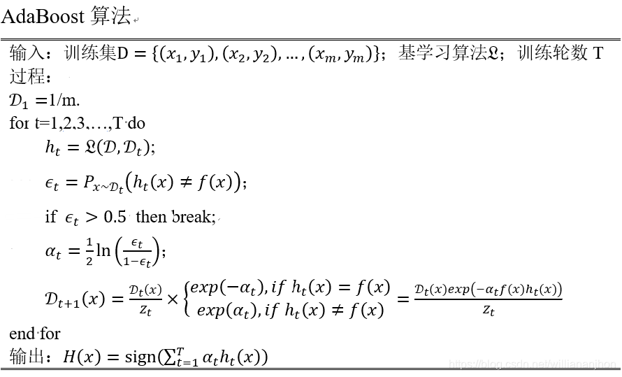
8.2 Boosting
Boosting是一族可将弱学习器提升为强学习器的算法。
工作机制
先从初始训练集训练出一个基学习器,再根据基学习器的表现对训练样本分布进行调整,使得先前基学习器做错的训练样本在后续受到更多关注,然后基于调整后的样本分布来训练下一个基学习器;如此重复进行,直至基学习器数目达到事先指定的值T,最终将这T个基学习器进行加权结合。
AdaBoost——加性模型(additive model)
基学习器的线性组合
H
(
x
)
=
∑
t
=
1
T
α
t
h
t
(
x
)
H\left( x \right) = \sum_{t = 1}^{T}{\alpha_{t}h_{t}\left( x \right)}
H
(
x
)
=
t
=
1
∑
T
α
t
h
t
(
x
)
最小化指数损失函数(exponential loss function)
l
exp
(
H
∣
D
)
=
E
x
∼
D
[
e
−
f
(
x
)
H
(
x
)
]
\mathcal{l}_{\exp}\left( H \middle| \mathcal{D} \right) = \mathbb{E}_{x\sim\mathcal{D}}\left\lbrack e^{- f\left( x \right)H\left( x \right)} \right\rbrack
l
exp
(
H
∣
D
)
=
E
x
∼
D
[
e
−
f
(
x
)
H
(
x
)
]
若
H
(
x
)
H\left( x \right)
H
(
x
)
能令指数损失函数最小化,则
∂
l
exp
(
H
∣
D
)
∂
H
(
x
)
=
−
e
−
H
(
x
)
P
(
f
(
x
)
=
1
∣
x
)
+
e
H
(
x
)
P
(
f
(
x
)
=
−
1
∣
x
)
\frac{\partial\mathcal{l}_{\exp}\left( H \middle| \mathcal{D} \right)}{\partial H\left( x \right)} = – e^{- H\left( x \right)}P\left( f\left( x \right) = 1 \middle| x \right) + e^{H\left( x \right)}P\left( f\left( x \right) = – 1 \middle| x \right)
∂
H
(
x
)
∂
l
exp
(
H
∣
D
)
=
−
e
−
H
(
x
)
P
(
f
(
x
)
=
1
∣
x
)
+
e
H
(
x
)
P
(
f
(
x
)
=
−
1
∣
x
)
令上式为0,可得
H
(
x
)
=
1
2
ln
P
(
f
(
x
)
=
1
∣
x
)
P
(
f
(
x
)
=
−
1
∣
x
)
H\left( x \right) = \frac{1}{2}\ln\frac{P\left( f\left( x \right) = 1 \middle| x \right)}{P\left( f\left( x \right) = – 1 \middle| x \right)}
H
(
x
)
=
2
1
ln
P
(
f
(
x
)
=
−
1
∣
x
)
P
(
f
(
x
)
=
1
∣
x
)
因此,有
sign
(
H
(
x
)
)
=
sign
(
1
2
ln
P
(
f
(
x
)
=
1
∣
x
)
P
(
f
(
x
)
=
−
1
∣
x
)
)
\text{sign}\left( H\left( x \right) \right) = \text{sign}\left( \frac{1}{2}\ln\frac{P\left( f\left( x \right) = 1 \middle| x \right)}{P\left( f\left( x \right) = – 1 \middle| x \right)} \right)
sign
(
H
(
x
)
)
=
sign
(
2
1
ln
P
(
f
(
x
)
=
−
1
∣
x
)
P
(
f
(
x
)
=
1
∣
x
)
)
=
{
1
,
P
(
f
(
x
)
=
1
∣
x
)
>
P
(
f
(
x
)
=
−
1
∣
x
)
−
1
,
P
(
f
(
x
)
=
1
∣
x
)
<
P
(
f
(
x
)
=
−
1
∣
x
)
= \left\{ \begin{matrix} 1,P\left( f\left( x \right) = 1 \middle| x \right) > P\left( f\left( x \right) = – 1 \middle| x \right) \\ – 1,P\left( f\left( x \right) = 1 \middle| x \right) < P\left( f\left( x \right) = – 1 \middle| x \right) \\ \end{matrix} \right.\
=
{
1
,
P
(
f
(
x
)
=
1
∣
x
)
>
P
(
f
(
x
)
=
−
1
∣
x
)
−
1
,
P
(
f
(
x
)
=
1
∣
x
)
<
P
(
f
(
x
)
=
−
1
∣
x
)
=
a
r
g
max
P
(
f
(
x
)
=
y
∣
x
)
= arg\operatorname{max}{P\left( f\left( x \right) = y \middle| x \right)}
=
a
r
g
m
a
x
P
(
f
(
x
)
=
y
∣
x
)
在AdaBoost算法中,第一个基学习器
h
1
h_{1}
h
1
是通过直接将基学习算法用于初始数据分布而得;此后迭代地生成
h
t
h_{t}
h
t
和
α
t
\alpha_{t}
α
t
,当基分类器
h
t
h_{t}
h
t
基于分布
D
t
\mathcal{D}_{t}
D
t
产生后,该基分类器的权重
α
t
\alpha_{t}
α
t
应使得
α
t
h
t
\alpha_{t}h_{t}
α
t
h
t
最小化指数损失函数
l
exp
(
α
t
h
t
∣
D
t
)
=
E
x
∼
D
t
[
e
−
f
(
x
)
α
t
h
t
(
x
)
]
\mathcal{l}_{\exp}\left( \alpha_{t}h_{t} \middle| \mathcal{D}_{t} \right) = \mathbb{E}_{x\sim\mathcal{D}_{t}}\left\lbrack e^{- f\left( x \right)\alpha_{t}h_{t}\left( x \right)} \right\rbrack
l
exp
(
α
t
h
t
∣
D
t
)
=
E
x
∼
D
t
[
e
−
f
(
x
)
α
t
h
t
(
x
)
]
=
E
x
∼
D
t
[
e
−
α
t
I
(
f
(
x
)
=
h
t
(
x
)
)
+
e
α
t
I
(
f
(
x
)
≠
h
t
(
x
)
)
]
= \mathbb{E}_{x\sim\mathcal{D}_{t}}\left\lbrack e^{- \alpha_{t}}\mathbb{I}\left( f\left( x \right) = h_{t}\left( x \right) \right) + e^{\alpha_{t}}\mathbb{I}\left( f\left( x \right) \neq h_{t}\left( x \right) \right) \right\rbrack
=
E
x
∼
D
t
[
e
−
α
t
I
(
f
(
x
)
=
h
t
(
x
)
)
+
e
α
t
I
(
f
(
x
)
̸
=
h
t
(
x
)
)
]
=
e
−
α
t
P
x
∼
D
t
(
f
(
x
)
=
h
t
(
x
)
)
+
e
α
t
P
x
∼
D
t
(
f
(
x
)
≠
h
t
(
x
)
)
= e^{- \alpha_{t}}P_{x\sim\mathcal{D}_{t}}\left( f\left( x \right) = h_{t}\left( x \right) \right) + e^{\alpha_{t}}P_{x\sim\mathcal{D}_{t}}\left( f\left( x \right) \neq h_{t}\left( x \right) \right)
=
e
−
α
t
P
x
∼
D
t
(
f
(
x
)
=
h
t
(
x
)
)
+
e
α
t
P
x
∼
D
t
(
f
(
x
)
̸
=
h
t
(
x
)
)
=
e
−
α
t
(
1
−
ϵ
t
)
+
e
α
t
ϵ
t
= e^{- \alpha_{t}}\left( 1 – \epsilon_{t} \right) + e^{\alpha_{t}}\epsilon_{t}
=
e
−
α
t
(
1
−
ϵ
t
)
+
e
α
t
ϵ
t
其中
ϵ
t
=
P
x
∼
D
t
(
f
(
x
)
≠
h
t
(
x
)
)
\epsilon_{t} = P_{x\sim\mathcal{D}_{t}}\left( f\left( x \right) \neq h_{t}\left( x \right) \right)
ϵ
t
=
P
x
∼
D
t
(
f
(
x
)
̸
=
h
t
(
x
)
)
。考虑指数损失函数的导数
∂
l
exp
(
α
t
h
t
∣
D
t
)
∂
α
t
=
−
e
−
α
t
(
1
−
ϵ
t
)
+
e
α
t
ϵ
t
\frac{\partial\mathcal{l}_{\exp}\left( \alpha_{t}h_{t} \middle| \mathcal{D}_{t} \right)}{\partial\alpha_{t}} = – e^{- \alpha_{t}}\left( 1 – \epsilon_{t} \right) + e^{\alpha_{t}}\epsilon_{t}
∂
α
t
∂
l
exp
(
α
t
h
t
∣
D
t
)
=
−
e
−
α
t
(
1
−
ϵ
t
)
+
e
α
t
ϵ
t
令上式等于0,得
分类器权重更新公式
α
t
=
1
2
ln
(
1
−
ϵ
t
ϵ
t
)
\alpha_{t} = \frac{1}{2}\ln\left( \frac{1 – \epsilon_{t}}{\epsilon_{t}} \right)
α
t
=
2
1
ln
(
ϵ
t
1
−
ϵ
t
)
理想的
h
t
h_{t}
h
t
能纠正
H
t
−
1
H_{t – 1}
H
t
−
1
的全部错误,即
l
exp
(
H
t
−
1
+
h
t
∣
D
)
=
E
x
∼
D
[
e
−
f
(
x
)
(
H
t
−
1
(
x
)
−
h
t
(
x
)
)
]
\mathcal{l}_{\exp}\left( H_{t – 1} + h_{t} \middle| \mathcal{D} \right) = \mathbb{E}_{x\sim\mathcal{D}}\left\lbrack e^{- f\left( x \right)\left( H_{t – 1}\left( x \right) – h_{t}\left( x \right) \right)} \right\rbrack
l
exp
(
H
t
−
1
+
h
t
∣
D
)
=
E
x
∼
D
[
e
−
f
(
x
)
(
H
t
−
1
(
x
)
−
h
t
(
x
)
)
]
E
x
∼
D
[
e
−
f
(
x
)
H
t
−
1
(
x
)
e
−
f
(
x
)
h
t
(
x
)
]
\mathbb{E}_{x\sim\mathcal{D}}\left\lbrack e^{- f\left( x \right)H_{t – 1}\left( x \right)}e^{- f\left( x \right)h_{t}\left( x \right)} \right\rbrack
E
x
∼
D
[
e
−
f
(
x
)
H
t
−
1
(
x
)
e
−
f
(
x
)
h
t
(
x
)
]
使用泰勒展式近似为
l
exp
(
H
t
−
1
+
h
t
∣
D
)
≃
E
x
∼
D
[
e
−
f
(
x
)
H
t
−
1
(
x
)
(
1
−
f
(
x
)
h
t
(
x
)
+
f
2
(
x
)
h
t
2
(
x
)
2
)
]
=
E
x
∼
D
[
e
−
f
(
x
)
H
t
−
1
(
x
)
(
1
−
f
(
x
)
h
t
(
x
)
+
1
2
)
]
\mathcal{l}_{\exp}\left( H_{t – 1} + h_{t} \middle| \mathcal{D} \right) \simeq \mathbb{E}_{x\sim\mathcal{D}}\left\lbrack e^{- f\left( x \right)H_{t – 1}\left( x \right)}\left( 1 – f\left( x \right)h_{t}\left( x \right) + \frac{f^{2}\left( x \right)h_{t}^{2}\left( x \right)}{2} \right) \right\rbrack = \mathbb{E}_{x\sim\mathcal{D}}\left\lbrack e^{- f\left( x \right)H_{t – 1}\left( x \right)}\left( 1 – f\left( x \right)h_{t}\left( x \right) + \frac{1}{2} \right) \right\rbrack
l
exp
(
H
t
−
1
+
h
t
∣
D
)
≃
E
x
∼
D
[
e
−
f
(
x
)
H
t
−
1
(
x
)
(
1
−
f
(
x
)
h
t
(
x
)
+
2
f
2
(
x
)
h
t
2
(
x
)
)
]
=
E
x
∼
D
[
e
−
f
(
x
)
H
t
−
1
(
x
)
(
1
−
f
(
x
)
h
t
(
x
)
+
2
1
)
]
理想学习器
h
t
(
x
)
=
arg
l
exp
(
H
t
−
1
+
h
∣
D
)
=
arg
E
x
∼
D
[
e
−
f
(
x
)
H
t
−
1
(
x
)
(
1
−
f
(
x
)
h
(
x
)
+
1
2
)
]
=
arg
E
x
∼
D
[
e
−
f
(
x
)
H
t
−
1
(
x
)
f
(
x
)
h
(
x
)
]
=
arg
E
x
∼
D
[
e
−
f
(
x
)
H
t
−
1
(
x
)
E
x
∼
D
[
e
−
f
(
x
)
H
t
−
1
(
x
)
]
f
(
x
)
h
(
x
)
]
h_{t}\left( x \right) = \arg\operatorname{}{\mathcal{l}_{\exp}\left( H_{t – 1} + h \middle| \mathcal{D} \right)} = \arg\operatorname{}{\mathbb{E}_{x\sim\mathcal{D}}\left\lbrack e^{- f\left( x \right)H_{t – 1}\left( x \right)}\left( 1 – f\left( x \right)h\left( x \right) + \frac{1}{2} \right) \right\rbrack} = \arg\operatorname{}{\mathbb{E}_{x\sim\mathcal{D}}\left\lbrack e^{- f\left( x \right)H_{t – 1}\left( x \right)}f\left( x \right)h\left( x \right) \right\rbrack = \arg\operatorname{}{\mathbb{E}_{x\sim\mathcal{D}}\left\lbrack \frac{e^{- f\left( x \right)H_{t – 1}\left( x \right)}}{\mathbb{E}_{x\sim\mathcal{D}}\left\lbrack e^{- f\left( x \right)H_{t – 1}\left( x \right)} \right\rbrack}f\left( x \right)h\left( x \right) \right\rbrack}}
h
t
(
x
)
=
ar
g
l
exp
(
H
t
−
1
+
h
∣
D
)
=
ar
g
E
x
∼
D
[
e
−
f
(
x
)
H
t
−
1
(
x
)
(
1
−
f
(
x
)
h
(
x
)
+
2
1
)
]
=
ar
g
E
x
∼
D
[
e
−
f
(
x
)
H
t
−
1
(
x
)
f
(
x
)
h
(
x
)
]
=
ar
g
E
x
∼
D
[
E
x
∼
D
[
e
−
f
(
x
)
H
t
−
1
(
x
)
]
e
−
f
(
x
)
H
t
−
1
(
x
)
f
(
x
)
h
(
x
)
]
注意到
E
x
∼
D
[
e
−
f
(
x
)
H
t
−
1
(
x
)
]
\mathbb{E}_{x\sim\mathcal{D}}\left\lbrack e^{- f\left( x \right)H_{t – 1}\left( x \right)} \right\rbrack
E
x
∼
D
[
e
−
f
(
x
)
H
t
−
1
(
x
)
]
是一个常数,令
D
t
\mathcal{D}_{t}
D
t
表示一个分布
D
t
(
x
)
=
D
(
x
)
e
−
f
(
x
)
H
t
−
1
(
x
)
E
x
∼
D
[
e
−
f
(
x
)
H
t
−
1
(
x
)
]
\mathcal{D}_{t}\left( x \right) = \frac{\mathcal{D}\left( x \right)e^{- f\left( x \right)H_{t – 1}\left( x \right)}}{\mathbb{E}_{x\sim\mathcal{D}}\left\lbrack e^{- f\left( x \right)H_{t – 1}\left( x \right)} \right\rbrack}
D
t
(
x
)
=
E
x
∼
D
[
e
−
f
(
x
)
H
t
−
1
(
x
)
]
D
(
x
)
e
−
f
(
x
)
H
t
−
1
(
x
)
则
h
t
(
x
)
=
arg
E
x
∼
D
[
e
−
f
(
x
)
H
t
−
1
(
x
)
E
x
∼
D
[
e
−
f
(
x
)
H
t
−
1
(
x
)
]
f
(
x
)
h
(
x
)
]
=
arg
E
x
∼
D
t
[
f
(
x
)
h
(
x
)
]
h_{t}\left( x \right) = \arg\operatorname{}{\mathbb{E}_{x\sim\mathcal{D}}\left\lbrack \frac{e^{- f\left( x \right)H_{t – 1}\left( x \right)}}{\mathbb{E}_{x\sim\mathcal{D}}\left\lbrack e^{- f\left( x \right)H_{t – 1}\left( x \right)} \right\rbrack}f\left( x \right)h\left( x \right) \right\rbrack} = \arg\operatorname{}{\mathbb{E}_{x\sim\mathcal{D}_{t}}\left\lbrack f\left( x \right)h\left( x \right) \right\rbrack}
h
t
(
x
)
=
ar
g
E
x
∼
D
[
E
x
∼
D
[
e
−
f
(
x
)
H
t
−
1
(
x
)
]
e
−
f
(
x
)
H
t
−
1
(
x
)
f
(
x
)
h
(
x
)
]
=
ar
g
E
x
∼
D
t
[
f
(
x
)
h
(
x
)
]
由
f
(
x
)
,
h
(
x
)
∈
{
−
1
,
1
}
f\left( x \right),h\left( x \right) \in \left\{ – 1,1 \right\}
f
(
x
)
,
h
(
x
)
∈
{
−
1
,
1
}
,有
f
(
x
)
h
(
x
)
=
1
−
2
I
(
f
(
x
)
≠
h
(
x
)
)
f\left( x \right)h\left( x \right) = 1 – 2\mathbb{I}\left( f\left( x \right) \neq h\left( x \right) \right)
f
(
x
)
h
(
x
)
=
1
−
2
I
(
f
(
x
)
̸
=
h
(
x
)
)
则理想的基学习器
h
t
(
x
)
=
arg
min
E
x
∼
D
t
[
I
(
f
(
x
)
≠
h
(
x
)
)
]
h_{t}\left( x \right) = \arg\operatorname{min}{\mathbb{E}_{x\sim\mathcal{D}_{t}}\left\lbrack \mathbb{I}\left( f\left( x \right) \neq h\left( x \right) \right) \right\rbrack}
h
t
(
x
)
=
ar
g
m
i
n
E
x
∼
D
t
[
I
(
f
(
x
)
̸
=
h
(
x
)
)
]
理想的
h
t
h_{t}
h
t
将在分布
D
t
\mathcal{D}_{t}
D
t
下最小化分类误差。考虑到
D
t
\mathcal{D}_{t}
D
t
和
D
t
+
1
\mathcal{D}_{t+ 1}
D
t
+
1
的关系,有样本分布更新公式:
D
t
+
1
=
D
(
x
)
e
−
f
(
x
)
H
t
(
x
)
E
x
∼
D
[
e
−
f
(
x
)
H
t
(
x
)
]
=
D
(
x
)
e
−
f
(
x
)
H
t
−
1
(
x
)
e
−
f
(
x
)
α
t
h
t
(
x
)
E
x
∼
D
[
e
−
f
(
x
)
H
t
(
x
)
]
=
D
t
(
x
)
∗
e
−
f
(
x
)
α
t
h
t
(
x
)
E
x
∼
D
[
e
−
f
(
x
)
H
t
−
1
(
x
)
]
E
x
∼
D
[
e
−
f
(
x
)
H
t
(
x
)
]
\mathcal{D}_{t + 1} = \frac{\mathcal{D}\left( x \right)e^{- f\left( x \right)H_{t}\left( x \right)}}{\mathbb{E}_{x\sim\mathcal{D}}\left\lbrack e^{- f\left( x \right)H_{t}\left( x \right)} \right\rbrack} = \frac{\mathcal{D}\left( x \right)e^{- f\left( x \right)H_{t – 1}\left( x \right)}e^{- f\left( x \right)\alpha_{t}h_{t}\left( x \right)}}{\mathbb{E}_{x\sim\mathcal{D}}\left\lbrack e^{- f\left( x \right)H_{t}\left( x \right)} \right\rbrack} = \mathcal{D}_{t}\left( x \right)*e^{- f\left( x \right)\alpha_{t}h_{t}\left( x \right)}\frac{\mathbb{E}_{x\sim\mathcal{D}}\left\lbrack e^{- f\left( x \right)H_{t – 1}\left( x \right)} \right\rbrack}{\mathbb{E}_{x\sim\mathcal{D}}\left\lbrack e^{- f\left( x \right)H_{t}\left( x \right)} \right\rbrack}
D
t
+
1
=
E
x
∼
D
[
e
−
f
(
x
)
H
t
(
x
)
]
D
(
x
)
e
−
f
(
x
)
H
t
(
x
)
=
E
x
∼
D
[
e
−
f
(
x
)
H
t
(
x
)
]
D
(
x
)
e
−
f
(
x
)
H
t
−
1
(
x
)
e
−
f
(
x
)
α
t
h
t
(
x
)
=
D
t
(
x
)
∗
e
−
f
(
x
)
α
t
h
t
(
x
)
E
x
∼
D
[
e
−
f
(
x
)
H
t
(
x
)
]
E
x
∼
D
[
e
−
f
(
x
)
H
t
−
1
(
x
)
]
8.3 Bagging与随机森林
8.3.1 Bagging
Bagging是并行式集成学习方法,基于自助采样法。
给定包含m个样本的数据集,先随机取出一个样本放入采样集中,再把该样本放回初始数据集。使得下次采样时该样本仍有可能被选中,经过m次随机采样操作,得到包含m个样本的采样集。
Bagging流程
采样T个含m个训练样本的采样集,然后基于每个采样集训练出一个基学习器,再将这些基学习器进行结合。
Bagging通常对分类任务使用简单投票法,对回归任务使用简单平均法。
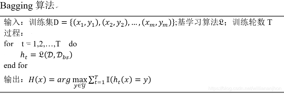
假定基学习器的计算复杂度为
O
(
m
)
O\left( m \right)
O
(
m
)
,则Bagging的复杂度大致为
T
(
O
(
m
)
+
O
(
s
)
)
T\left( O\left( m \right) + O\left( s \right) \right)
T
(
O
(
m
)
+
O
(
s
)
)
令
D
t
\mathcal{D}_{t}
D
t
表示
h
t
(
x
)
h_{t}\left( x \right)
h
t
(
x
)
实际使用的训练样本集,令
H
oob
(
x
)
H^{\text{oob}}\left( x \right)
H
oob
(
x
)
表示对样本的包外预测,即仅考虑那些未使用x训练的基学习器在x上的预测,有
H
oob
(
x
)
=
arg
max
∑
t
=
1
T
I
(
h
t
(
x
)
=
y
)
∗
I
(
x
∉
D
t
)
H^{\text{oob}}\left( x \right) = \arg\operatorname{max}{\sum_{t = 1}^{T}{\mathbb{I}\left( h_{t}\left( x \right) = y \right)}}\mathbb{*I}\left( x \notin \mathcal{D}_{t} \right)
H
oob
(
x
)
=
ar
g
m
a
x
t
=
1
∑
T
I
(
h
t
(
x
)
=
y
)
∗
I
(
x
∈
/
D
t
)
则Bagging泛化误差的包外估计为
ϵ
oob
=
1
∣
D
∣
∑
(
x
,
y
)
∈
D
I
(
H
oob
(
x
)
≠
y
)
\epsilon^{\text{oob}} = \frac{1}{\left| \mathcal{D} \right|}\sum_{\left( x,y \right)\mathcal{\in D}}^{}{\mathbb{I}\left( H^{\text{oob}}\left( x \right) \neq y \right)}
ϵ
oob
=
∣
D
∣
1
(
x
,
y
)
∈
D
∑
I
(
H
oob
(
x
)
̸
=
y
)
8.3.2 随机森林
随机森林
(Random Forest,RF)是Bagging的一个扩展变体。RF在以决策树为基础学习器构建Bagging基础的基础上,进一步在决策树的训练过程中引入随机属性选择。
RF
对基决策树的每个结点,先从该结点的属性集合中随机选择一个包含k个属性的子集,然后再从这个子集中选择一个最优属性用于划分。一般情况下,参数
k
=
d
k= \operatorname{}d
k
=
d
优点:随机森林简单、容易实现、计算开销小。
8.4 结合策略
学习器结合的好处
1、减小单学习器泛化性能不佳的风险
2、降低陷入糟糕局部极小点的风险
3、扩大假设空间
8.4.1 平均法
简单平均法(simple average)
H
(
x
)
=
1
T
∑
i
=
1
T
h
i
(
x
)
H\left( x \right) = \frac{1}{T}\sum_{i = 1}^{T}{h_{i}\left( x \right)}
H
(
x
)
=
T
1
i
=
1
∑
T
h
i
(
x
)
加权平均法
H
(
x
)
=
∑
i
=
1
T
ω
i
h
i
(
x
)
H\left( x \right) = \sum_{i = 1}^{T}{\omega_{i}h_{i}\left( x \right)}
H
(
x
)
=
i
=
1
∑
T
ω
i
h
i
(
x
)
其中
ω
i
\omega_{i}
ω
i
是个体学习器
h
i
h_{i}
h
i
的权重,通常要求
ω
i
≥
0
,
∑
i
=
1
T
ω
i
=
1
\omega_{i} \geq 0,\sum_{i = 1}^{T}\omega_{i} = 1
ω
i
≥
0
,
∑
i
=
1
T
ω
i
=
1
集成学习研究的基本出发点,对给定的基学习器,不同的集成学习方法可视为通过不同的方式来确定加权平均法中的基学习器权重。
8.4.2 投票法
学习器
h
i
h_{i}
h
i
将从类别集合
{
c
1
,
c
2
,
…
,
c
N
}
\left\{ c_{1},c_{2},\ldots,c_{N} \right\}
{
c
1
,
c
2
,
…
,
c
N
}
中预测出一个标记,将
h
i
h_{i}
h
i
在样本x上的预测输出表示为一个N维向量
(
h
i
1
(
x
)
;
h
i
2
(
x
)
;
…
;
h
i
N
(
x
)
)
\left( h_{i}^{1}\left( x \right);h_{i}^{2}\left( x \right);\ldots;h_{i}^{N}\left( x \right) \right)
(
h
i
1
(
x
)
;
h
i
2
(
x
)
;
…
;
h
i
N
(
x
)
)
,其中
h
i
j
(
x
)
h_{i}^{j}\left( x \right)
h
i
j
(
x
)
是
h
i
h_{i}
h
i
在类别标记
c
j
c_{j}
c
j
上的输出
绝对多数投票法(majority voting)
H
(
x
)
=
{
c
j
,
i
f
∑
i
=
1
T
h
i
j
(
x
)
>
0.5
∑
k
=
1
N
∑
i
=
1
T
h
i
k
(
x
)
reject
,
o
t
h
e
r
w
i
s
e
H\left( x \right) = \left\{ \begin{matrix} c_{j},if\ \sum_{i = 1}^{T}h_{i}^{j}\left( x \right) > 0.5\sum_{k = 1}^{N}{\sum_{i = 1}^{T}{h_{i}^{k}\left( x \right)}} \\\text{reject},otherwise \\\end{matrix} \right.\
H
(
x
)
=
{
c
j
,
i
f
∑
i
=
1
T
h
i
j
(
x
)
>
0
.
5
∑
k
=
1
N
∑
i
=
1
T
h
i
k
(
x
)
reject
,
o
t
h
e
r
w
i
s
e
即若某标记得票过半数,则预测为该标记,否则拒绝预测。
相对多数投票法(plurality voting)
H
(
x
)
=
c
arg
max
∑
i
=
1
T
h
i
j
(
x
)
H\left( x \right) = c_{\arg\operatorname{max}{\sum_{i = 1}^{T}h_{i}^{j}\left( x \right)}}
H
(
x
)
=
c
ar
g
m
a
x
∑
i
=
1
T
h
i
j
(
x
)
即预测为得票最多的标记,若同时有多个标记获最高票,则从中随机选取一个。
加权投票法(weighted voting)
H
(
x
)
=
c
arg
max
∑
i
=
1
T
ω
i
h
i
j
(
x
)
H\left( x \right) = c_{\arg\operatorname{max}{\sum_{i = 1}^{T}{\omega_{i}h_{i}^{j}}\left( x \right)}}
H
(
x
)
=
c
ar
g
m
a
x
∑
i
=
1
T
ω
i
h
i
j
(
x
)
其中
ω
i
\omega_{i}
ω
i
是个体学习器
h
i
h_{i}
h
i
的权重,通常要求
ω
i
≥
0
,
∑
i
=
1
T
ω
i
=
1
\omega_{i} \geq 0,\sum_{i = 1}^{T}\omega_{i} = 1
ω
i
≥
0
,
∑
i
=
1
T
ω
i
=
1
硬投票(hard voting)
:类标记
h
i
j
(
x
)
∈
{
0.1
}
h_{i}^{j}\left( x \right) \in \left\{ 0.1 \right\}
h
i
j
(
x
)
∈
{
0
.
1
}
,若
h
i
h_{i}
h
i
将样本x预测为类别
c
j
c_{j}
c
j
则取值为1,否则为0。
软投票(soft voting)
:类概率
h
i
j
(
x
)
∈
[
0
,
1
]
h_{i}^{j}\left( x \right) \in \left\lbrack 0,1 \right\rbrack
h
i
j
(
x
)
∈
[
0
,
1
]
,若
h
i
h_{i}
h
i
将样本x预测为类别
c
j
c_{j}
c
j
则取值为1,否则为0。
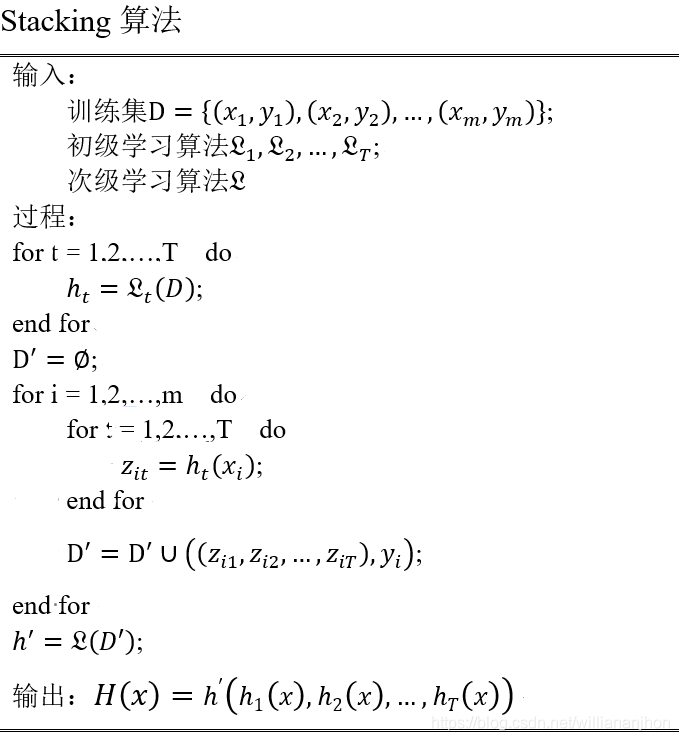
8.4.3 学习法
通过另一个学习器来进行结合。把个体学习器称为初级学习器,用于结合的学习器称为次级学习器或元学习器(meta-learner)
8.5 多样性
8.5.1 误差-分歧分解
假定用个体学习器
h
1
,
h
2
,
…
,
h
T
h_{1},h_{2},\ldots,h_{T}
h
1
,
h
2
,
…
,
h
T
通过加权平均法结合产生的集成来完成回归学习任务
f
:
R
d
→
R
f:\mathbb{R}^{d}\mathbb{\rightarrow R}
f
:
R
d
→
R
。对示例x,定义学习器
h
i
h_{i}
h
i
的分歧(ambiguity)为
A
(
h
i
∣
x
)
=
(
h
i
(
x
)
−
H
(
x
)
)
2
A\left( h_{i} \middle| x \right) = \left( h_{i}\left( x \right) – H\left( x \right) \right)^{2}
A
(
h
i
∣
x
)
=
(
h
i
(
x
)
−
H
(
x
)
)
2
则集成的分歧为
A
‾
(
h
∣
x
)
=
∑
i
=
1
T
ω
i
A
(
h
i
∣
x
)
=
∑
i
=
1
T
ω
i
(
h
i
(
x
)
−
H
(
x
)
)
2
\overset{\overline{}}{A}\left( h \middle| x \right) = \sum_{i = 1}^{T}\omega_{i}A\left( h_{i} \middle| x \right) = \sum_{i = 1}^{T}{\omega_{i}\left( h_{i}\left( x \right) – H\left( x \right) \right)^{2}}
A
(
h
∣
x
)
=
i
=
1
∑
T
ω
i
A
(
h
i
∣
x
)
=
i
=
1
∑
T
ω
i
(
h
i
(
x
)
−
H
(
x
)
)
2
分歧项表征了个体学习器在样本x上的不一致性。个体学习器
h
i
h_{i}
h
i
和集成H的平方误差分别为
E
(
h
i
∣
x
)
=
(
f
(
x
)
−
h
i
(
x
)
)
2
E\left( h_{i} \middle| x \right) = \left( f\left( x \right) – h_{i}\left( x \right) \right)^{2}
E
(
h
i
∣
x
)
=
(
f
(
x
)
−
h
i
(
x
)
)
2
E
(
h
∣
x
)
=
(
f
(
x
)
−
H
(
x
)
)
2
E\left( h \middle| x \right) = \left( f\left( x \right) – H\left( x \right) \right)^{2}
E
(
h
∣
x
)
=
(
f
(
x
)
−
H
(
x
)
)
2
令
E
‾
(
h
∣
x
)
=
∑
i
=
1
T
ω
i
E
(
h
i
∣
x
)
\overset{\overline{}}{E}\left( h \middle| x \right) = \sum_{i = 1}^{T}{\omega_{i}E\left( h_{i} \middle| x \right)}
E
(
h
∣
x
)
=
∑
i
=
1
T
ω
i
E
(
h
i
∣
x
)
表示个体学习器误差的加权均值,有
A
‾
(
h
∣
x
)
=
∑
i
=
1
T
ω
i
E
(
h
i
∣
x
)
−
E
(
H
∣
x
)
=
E
‾
(
h
∣
x
)
−
E
(
H
∣
x
)
\overset{\overline{}}{A}\left( h \middle| x \right) = \sum_{i = 1}^{T}{\omega_{i}E\left( h_{i} \middle| x \right) -}E\left( H \middle| x \right) = \overset{\overline{}}{E}\left( h \middle| x \right) – E\left( H \middle| x \right)
A
(
h
∣
x
)
=
i
=
1
∑
T
ω
i
E
(
h
i
∣
x
)
−
E
(
H
∣
x
)
=
E
(
h
∣
x
)
−
E
(
H
∣
x
)
令
p
(
x
)
p\left( x \right)
p
(
x
)
表示样本的概率密度,则在全样本上有
∑
i
=
1
T
ω
i
∫
A
(
h
i
∣
x
)
p
(
x
)
dx
=
∑
i
=
1
T
ω
i
∫
E
(
h
i
∣
x
)
p
(
x
)
d
x
−
∫
E
(
H
∣
x
)
p
(
x
)
dx
\sum_{i = 1}^{T}{\omega_{i}\int_{}^{}{A\left( h_{i} \middle| x \right)p\left( x \right)}}\text{dx} = \sum_{i = 1}^{T}{\omega_{i}\int_{}^{}{E\left( h_{i} \middle| x \right)p\left( x \right)}}dx – \int_{}^{}{E\left( H \middle| x \right)p\left( x \right)\text{dx}}
i
=
1
∑
T
ω
i
∫
A
(
h
i
∣
x
)
p
(
x
)
dx
=
i
=
1
∑
T
ω
i
∫
E
(
h
i
∣
x
)
p
(
x
)
d
x
−
∫
E
(
H
∣
x
)
p
(
x
)
dx
个体学习器
h
i
h_{i}
h
i
在全样本上的泛化误差和分歧项分别为
E
i
=
∫
E
(
h
i
∣
x
)
p
(
x
)
dx
E_{i} = \int_{}^{}{E\left( h_{i} \middle| x \right)p\left( x \right)\text{dx}}
E
i
=
∫
E
(
h
i
∣
x
)
p
(
x
)
dx
A
i
=
∫
A
(
h
i
∣
x
)
p
(
x
)
dx
A_{i} = \int_{}^{}{A\left( h_{i} \middle| x \right)p\left( x \right)\text{dx}}
A
i
=
∫
A
(
h
i
∣
x
)
p
(
x
)
dx
集成的泛化误差为
E
=
∫
E
(
H
∣
x
)
p
(
x
)
dx
E = \int_{}^{}{E\left( H \middle| x \right)p\left( x \right)\text{dx}}
E
=
∫
E
(
H
∣
x
)
p
(
x
)
dx
再令
E
‾
=
∑
i
=
1
T
ω
i
E
i
\overset{\overline{}}{E} = \sum_{i = 1}^{T}{\omega_{i}E_{i}}
E
=
∑
i
=
1
T
ω
i
E
i
表示个体学习器泛化误差的加权均值,
A
‾
=
∑
i
=
1
T
ω
i
A
i
\overset{\overline{}}{A} = \sum_{i = 1}^{T}{\omega_{i}A_{i}}
A
=
∑
i
=
1
T
ω
i
A
i
表示个体学习器的加权分歧值,有
E
=
E
‾
−
A
‾
E = \overset{\overline{}}{E} – \overset{\overline{}}{A}
E
=
E
−
A
个体学习器准确性越高、多样性越大,则集成越好。
8.5.2 多样性度量
多样性度量(diversity measure)是用于度量集成中个体分类器的多样性。即估计个体学习器的多样化程度。
给定数据集
D
=
{
(
x
1
,
y
1
)
,
(
x
2
,
y
2
)
,
…
,
(
x
m
,
y
m
)
}
D = \left\{ \left( x_{1},y_{1} \right),\left( x_{2},y_{2} \right),\ldots,\left( x_{m},y_{m} \right) \right\}
D
=
{
(
x
1
,
y
1
)
,
(
x
2
,
y
2
)
,
…
,
(
x
m
,
y
m
)
}
,对二分类任务,
y
i
∈
{
−
1
,
1
}
y_{i} \in \left\{ – 1,1 \right\}
y
i
∈
{
−
1
,
1
}
,分类器
h
i
h_{i}
h
i
和
h
j
h_{j}
h
j
的预测结果列联表(contingency table)为
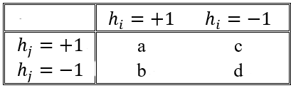
其中,a表示
h
i
h_{i}
h
i
和
h
j
h_{j}
h
j
均预测为正类的样本数目;b、c、d含义由此类推;
a
+
b
+
c
+
d
=
m
a+ b + c + d = m
a
+
b
+
c
+
d
=
m
不合度量(disagreement measure)
dis
ij
=
b
+
c
m
\text{dis}_{\text{ij}} = \frac{b + c}{m}
dis
ij
=
m
b
+
c
dis
ij
\text{dis}_{\text{ij}}
dis
ij
的值域为
[
0
,
1
]
\left\lbrack 0,1 \right\rbrack
[
0
,
1
]
,值越大则多样性越大。
相关系数(correlation coefficient)
ρ
ij
=
a
d
−
b
c
(
a
+
b
)
(
a
+
c
)
(
c
+
d
)
(
b
+
d
)
\rho_{\text{ij}} = \frac{ad – bc}{\sqrt{\left( a + b \right)\left( a + c \right)\left( c + d \right)\left( b + d \right)}}
ρ
ij
=
(
a
+
b
)
(
a
+
c
)
(
c
+
d
)
(
b
+
d
)
a
d
−
b
c
ρ
ij
\rho_{\text{ij}}
ρ
ij
的值域为
[
−
1
,
1
]
\left\lbrack – 1,1 \right\rbrack
[
−
1
,
1
]
,若
h
i
h_{i}
h
i
和
h
j
h_{j}
h
j
无关,则值为0;若
h
i
h_{i}
h
i
和
h
j
h_{j}
h
j
正相关则值为正,否则为负。
Q-统计量(Q-statistic)
Q
ij
=
a
d
−
b
c
a
d
+
b
c
Q_{\text{ij}} = \frac{ad – bc}{ad + bc}
Q
ij
=
a
d
+
b
c
a
d
−
b
c
Q
ij
Q_{\text{ij}}
Q
ij
与相关系数
ρ
ij
\rho_{\text{ij}}
ρ
ij
的符号相同,且
∣
Q
ij
∣
>
∣
ρ
ij
∣
\left| Q_{\text{ij}} \right| > \left| \rho_{\text{ij}} \right|
∣
Q
ij
∣
>
∣
ρ
ij
∣
K
\mathcal{K}
K
-统计量(
K
\mathcal{K}
K
-statistic)
K
=
p
1
−
p
2
1
−
p
2
\mathcal{K}\mathbf{=}\frac{p_{1} – p_{2}}{1 – p_{2}}
K
=
1
−
p
2
p
1
−
p
2
其中,
p
1
p_{1}
p
1
是两个分类器取得一致的概率;
p
2
p_{2}
p
2
是两个分类器偶然达成一致的概率,由数据集D估算:
p
1
=
a
+
d
m
p_{1} = \frac{a + d}{m}
p
1
=
m
a
+
d
p
2
=
(
a
+
b
)
(
a
+
c
)
+
(
c
+
d
)
(
b
+
d
)
m
2
p_{2} = \frac{\left( a + b \right)\left( a + c \right) + \left( c + d \right)\left( b + d \right)}{m^{2}}
p
2
=
m
2
(
a
+
b
)
(
a
+
c
)
+
(
c
+
d
)
(
b
+
d
)
若
h
i
h_{i}
h
i
和
h
j
h_{j}
h
j
在D上完全一致,则
K
=
1
\mathcal{K} = 1
K
=
1
;若
h
i
h_{i}
h
i
和
h
j
h_{j}
h
j
偶尔达成一致,则
K
=
0
\mathcal{K} = 0
K
=
0
;
K
\mathcal{K}
K
通常为非负值。
8.5.3 多样性增强
数据样本扰动
通常是基于采样法,此类做法简单高效,使用最广。
输入属性扰动
训练样本通常由一组属性描述,不同的子空间提供了观察数据的不同视角。
随机子空间(random subspace)算法
:依赖于输入属性扰动,该算法从初始属性集中抽取若干个属性子集,再基于每个属性子集训练一个基学习器。

输出表示扰动
基本思想:对输出表示进行操纵以增强多样性。
算法参数扰动
基学习算法一般都有参数需进行设置,通过随机设置不同的参数,往往可产生差别较大的个体学习器。