Logistic回归
0、读取数据
def read_dataset(filename, type_tuple, separator=','):
    with open(filename) as f:
        lines = f.readlines()
        data = []
        for line in lines:
            line = line[:-1]
            line = line.split(sep=separator)
            row = []
            for i in range(len(line)):
                row.append(type_tuple[i](line[i]))
            data.append(row)
        return np.array(data)
1、将数据进行二分类
def separate_dataset(data, col, boundary):
    data0 = np.array(data)
    data1 = np.array(data)
    dc0, dc1 = 0, 0
    for i in range(data.shape[0]):
        # 为1的数据
        if data[i][col] < boundary:
            data1 = np.delete(data1, i-dc1, axis=0)
            dc1 += 1
        # 为0的数据
        else:
            data0 = np.delete(data0, i-dc0, axis=0)
            dc0 += 1
    return data0, data1
2、画图验证
    data = read_dataset(文件路径, (float, float, float), separator=',')
    data0, data1 = separate_dataset(data, -1, 0.5)

    # 画图
    plt.title("raw data scatter")
    plt.xlabel("exam1 score")
    plt.ylabel("exam2 score")
    plt.scatter(data0[:, 0], data0[:, 1], marker='o', c='y', label="not admitted")
    plt.scatter(data1[:, 0], data1[:, 1], marker='x', c='b', label="admitted")
    plt.legend()
    plt.show()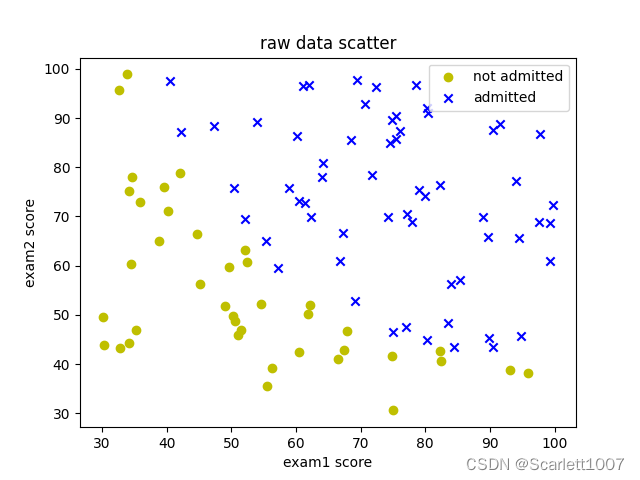
3、实现代价函数和梯度下降
def sigmoid(z):
    return 1/(1+np.exp(-z))


def cost(theta, X, y):
    return np.mean(-y*np.log(sigmoid(X.dot(theta)))-(1-y)*np.log(1-sigmoid(X.dot(theta))))
    # 等价于
    # return (-y.dot(np.log(sigmoid(X.dot(theta))))-(1-y).dot(np.log(1-sigmoid(X.dot(theta)))))/y.shape[0]


def gradient(theta, X, y):
    return X.T.dot(sigmoid(X.dot(theta))-y)/y.shape[0]

def gradient_descent(X, y, theta, alpha, iterations):
    for i in range(iterations):
        theta -= alpha*gradient(theta, X, y)
    return theta
4、测试代价函数和梯度下降
    # 测试代价函数, theta初始值取0
    data = np.array(data)
    X = np.insert(data[:, :-1], 0, 1, axis=1)
    y = data[:, 2]
    theta = np.zeros((3,))
    print(cost(theta, X, y))
    # 输出:0.6931471805599453

    # 特征归一化
    mean = np.mean(X[:, 1:], axis=0)
    std = np.std(X[:, 1:], axis=0, ddof=1)
    X[:, 1:] = (X[:, 1:]-mean)/std

    # 梯度下降
    alpha = 0.2
    iterations = 10000
    theta = gradient_descent(X, y, theta, alpha, iterations)
    print("theta:", theta)
    # 输出:theta: [1.71844349 4.01288964 3.74389058]
5、利用优化算法
    # 使用scipy中的高级优化算法
    res = opt.minimize(fun=cost, x0=theta, args=(X, y), method="TNC", jac=gradient)
    theta = res.x
    print("使用优化算法theta:", res.x)
    # 输出:使用优化算法theta: [1.71844349 4.01288964 3.74389058]
6、画出决策边界
    # 画出决策边界
    x1 = np.arange(20,110,0.1)
    # 进行了特征缩放,所以要还原
    x2 = mean[1] - std[1] * (theta[0] + theta[1] * (x1 - mean[0]) / std[0]) / theta[2]
    fig, ax = plt.subplots()
    ax.plot(x1, x2, 'r', label='decision boundary')
    ax.scatter(data0[:, 0], data0[:, 1], marker='o', c='y', label="not admitted")
    ax.scatter(data1[:, 0], data1[:, 1], marker='x', c='b', label="admitted")
    plt.legend()
    plt.show()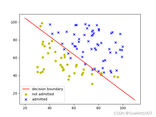
7、测试优化结果
    def predict(theta, X):
    return 1 if sigmoid(X.dot(theta)) > 0.6 else 0


    # 如果学生exam1得分45,exam2得分85
    test_s = np.array([45, 85])
    test_s = (test_s - mean)/std
    test_s = np.insert(test_s, 0, 1)
    print(sigmoid(test_s.dot(theta)))
    print(predict(theta, test_s))
    # 输出:0.7762898358371403
           1
正则化Logistic
0、导入需要的库
import numpy as np
import matplotlib.pyplot as plt
import scipy.optimize as opt
from sklearn.metrics import classification_report
1、读取数据并分类
# 读取数据
def read_dataset(filename, type_tuple, separator=','):
    with open(filename) as f:
        lines = f.readlines()
        data = []
        for line in lines:
            line = line[:-1]
            line = line.split(sep=separator)
            row = []
            for i in range(len(line)):
                row.append(type_tuple[i](line[i]))
            data.append(row)
        return np.array(data)


# 数据分类
def separate_dataset(data, col, boundary):
    data0, data1 = [], []
    for i in range(data.shape[0]):
        if data[i][col] < boundary:
            data0.append(data[i])
        else:
            data1.append(data[i])
    data0 = np.array(data0)
    data1 = np.array(data1)
    return data0, data1
2、画图验证
data = read_dataset(文件路径, (float, float, float), separator=',')
    data0, data1 = separate_dataset(data, -1, 0.5)

    # 画图
    plt.title("raw data scatter")
    plt.xlabel("exam1 score")
    plt.ylabel("exam2 score")
    plt.scatter(data0[:, 0], data0[:, 1], marker='x', c='y', label="not admitted")
    plt.scatter(data1[:, 0], data1[:, 1], marker='o', c='b', label="admitted")
    plt.legend()
    plt.show()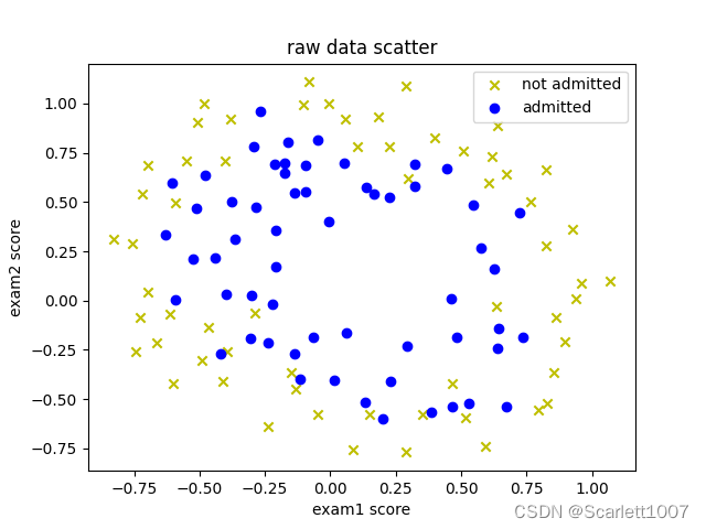
3、特征映射
# 特征映射
def features_mapping(x1, x2, power):
    m = len(x1)
    features = np.zeros((m, 1))
    for sum_power in range(power):
        for x1_power in range(sum_power+1):
            x2_power = sum_power - x1_power
            features = np.concatenate((features, (np.power(x1, x1_power)*np.power(x2, x2_power)).reshape(m, 1)), axis=1)
    return np.delete(features, 0, axis=1)
4、代价函数及梯度下降
def sigmoid(z):
    return 1/(1+np.exp(-z))


def cost(theta, X, y, lamda):
    m = X.shape[0]
    part1 = np.mean(-y*np.log(sigmoid(X.dot(theta)))-(1-y)*np.log(1-sigmoid(X.dot(theta))))
    part2 = (lamda/(2*m))*np.sum(np.delete((theta*theta), 0, axis=0))
    return part1+part2


def gradient(theta, X, y, lamda):
    m = X.shape[0]
    part1 = X.T.dot(sigmoid(X.dot(theta))-y)/y.shape[0]
    part2 = (lamda/m)*theta
    return part1+part2
5、代入数据验证
    # 特征映射
    features = features_mapping(data[:, 0], data[:, 1], 6)

    # 打印代价函数
    y = data[:, -1]
    theta = np.zeros(features.shape[-1])
    print(cost(theta, features, y, 1))
    #输出:0.6931471805599454
6、优化算法并检验预测情况
def predict(theta, X):
    return [1 if i > 0.5 else 0 for i in sigmoid(X.dot(theta))]

# 优化算法
    res = opt.minimize(fun=cost, x0=theta, args=(features, y, 1), method="TNC", jac=gradient)
    theta1 = res.x
    print(classification_report(y, predict(theta1, features)))
    # 输出:  precision    recall  f1-score   support

         0.0       0.85      0.77      0.81        60
         1.0       0.78      0.86      0.82        58

    accuracy                           0.81       118
   macro avg       0.82      0.81      0.81       118
weighted avg       0.82      0.81      0.81       118
7、画出决策边界
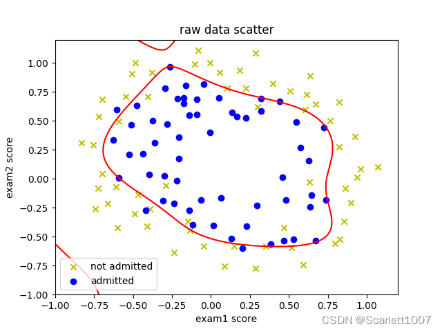
x = np.linspace(-1, 1.2, 100)
x1, x2 = np.meshgrid(x, x)
z = features_mapping(x1.ravel(), x2.ravel(), 6)
z = z.dot(res.x).reshape(x1.shape)
db = plt.contour(x1, x2, z, 0, colors=['r'])
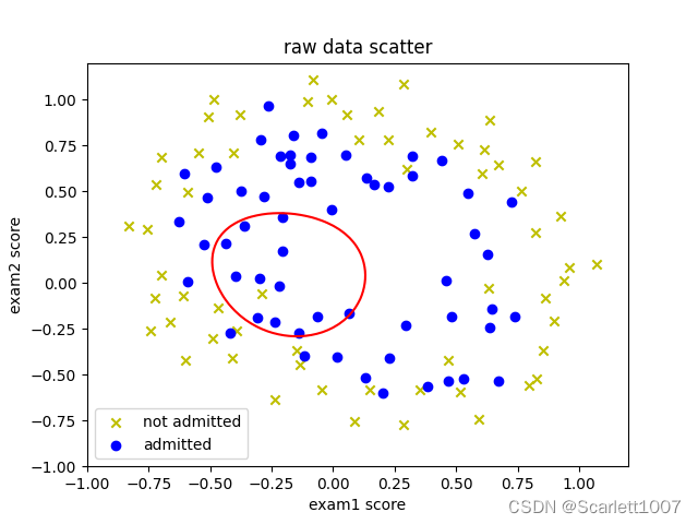
plt.title("raw data scatter")
plt.xlabel("exam1 score")
plt.ylabel("exam2 score")
plt.scatter(data0[:, 0], data0[:, 1], marker='x', c='y', label="not admitted")
plt.scatter(data1[:, 0], data1[:, 1], marker='o', c='b', label="admitted")
plt.legend()
plt.show()lamda=1时:
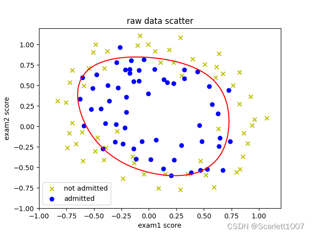
lamda=0时:
lamda=100时
版权声明:本文为weixin_59057086原创文章,遵循 CC 4.0 BY-SA 版权协议,转载请附上原文出处链接和本声明。