博客

RNN实现分类问题

import torch
import torch.nn as nn
from torch.autograd import Variable
import torchvision.datasets as dsets #包括了一些数据库，图片的数据库也包含了
import torchvision.transforms as transforms
import matplotlib.pyplot as plt

#超参数
EPOCH = 1
BATCH_SIZE = 64
TIME_STEP = 28  #rnn time step-->image height
INPUT_SIZE = 28  #rnn input size-->image width
LR = 0.01
DOWNLOAD_MNIST = False #已经下载好了，download设置成false



#准备训练数据
train_data = dsets.MNIST(
        root = r'D:\python\minist', #存储路径
        train = True,
        transform = transforms.ToTensor(), #把下载的数据改成Tensor形式
        #把(0-255)转换成(0-1)
        download = DOWNLOAD_MNIST #如果没下载就确认下载,如果已经下载了就填False
        )
#把train_data变成train_loader，训练起来比较有效率
train_loader = torch.utils.data.DataLoader(dataset = train_data,batch_size = BATCH_SIZE,shuffle = True)




#准备测试数据
test_data = dsets.MNIST(
        root = r'D:\python\minist', #存储路径
        train = False, #提取测试集不是训练集了
        transform = transforms.ToTensor(), #把下载的数据改成Tensor形式
        #把(0-255)转换成(0-1)
        )

test_x = Variable(test_data.test_data,volatile = True).type(torch.FloatTensor)[:2000]/255
test_y = test_data.test_labels.squeeze()[:2000]


#建立RNN神经网路
class RNN(nn.Module):
    def __init__(self):
        super(RNN,self).__init__()
        self.rnn = nn.LSTM(     #nn.RNN没有nn.LSTM效果好，收敛快
                input_size = INPUT_SIZE,
                hidden_size = 64,
                num_layers = 1, #中间只有一层神经层
                batch_first = True, #把batch_size参数放在第一个维度(batch,time_step,input)
                )
        self.out = nn.Linear(64,10)
        
    #三维数据展平成2维数据
    def forward(self,x):
        r_out,(h_n,h_c) = self.rnn(x,None)  #x-->(batch,time_step,input_size)
        #在这里分类问题不涉及(h_n,h_c),传入的是None
        out = self.out(r_out[:,-1,:]) #r_out-->(batch,time_step,input)
        #选取最后一个时间的out作为评价
        return out

rnn = RNN()
print(rnn)

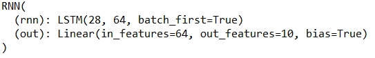
RNN网络只有一个LSTM层一个输出层，LSTM有64个神经元

#优化器
optimizer = torch.optim.Adam(rnn.parameters(),lr = LR)#优化器
loss_func = nn.CrossEntropyLoss()#计算损失函数
#CrossEntropy在torch中定义的不是onehot类型的，是int型的标签，标签是7就是7

#训练过程
for epoch in range(EPOCH):
    for step, (x,y) in enumerate(train_loader):   # 分配 batch data, normalize x when iterate train_loader
        b_x = Variable(x.view(-1,28,28)) #reshape x to (batch,time_step,input_size)
        #view设置不能缺参数，设置为-1表示自动判断，给出后面两维的大小28,28，自动判断前面的数
        b_y = Variable(y) #batch y
        output = rnn(b_x)
        loss = loss_func(output,b_y)
        optimizer.zero_grad()
        loss.backward()
        optimizer.step()
        
        #打印出来训练效果
        if step % 50 == 0:
            test_output = rnn(test_x)
            pred_y = torch.max(test_output,1)[1].data.numpy().squeeze()
            accuracy = float((pred_y == test_y).sum()) / float(test_y.size(0))
            #算括号里的是否等于，等于表示预测对了记一次，总共对的次数除以总数就是accuracy
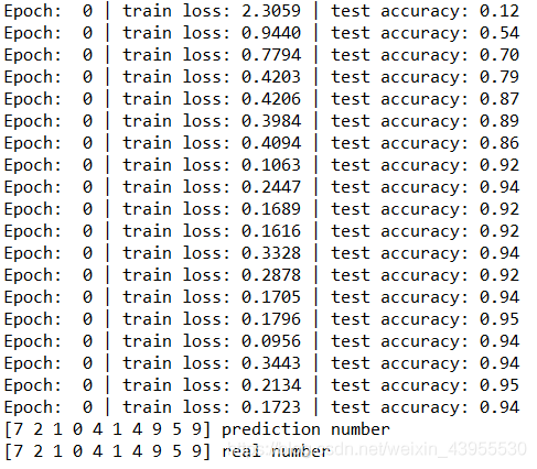
            print('Epoch: ',epoch,'| train loss: %.4f' % loss.data[0],'| test accuracy: %.2f' % accuracy)
        

#拿测试集前十个数据测试一下效果
test_output = rnn(test_x[:10].view(-1,28,28))
pred_y = torch.max(test_output,1)[1].data.numpy().squeeze()
print(pred_y,'prediction number')
print(test_y[:10].numpy(),'real number')

RNN实现回归问题

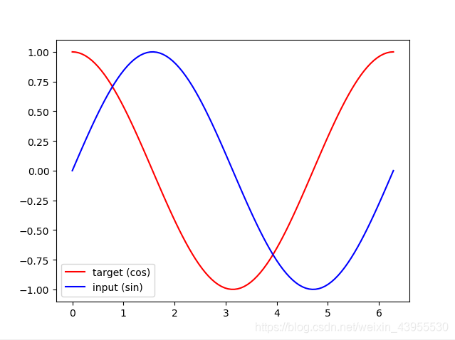
目标是给出一个sin分布的值，来预测一个cos分布的值，就是给出sin上面的一个y值，预测cos上面的值是多少

import torch
from torch import nn
from torch.autograd import Variable
import numpy as np
import matplotlib.pyplot as plt

# Hyper Parameters
TIME_STEP = 10      # rnn time step
INPUT_SIZE = 1      # rnn input size
LR = 0.02           # learning rate

## show data
#steps = np.linspace(0, np.pi*2, 100, dtype=np.float32)  # float32 for converting torch FloatTensor
#x_np = np.sin(steps)
#y_np = np.cos(steps)
#plt.plot(steps, y_np, 'r-', label='target (cos)')
#plt.plot(steps, x_np, 'b-', label='input (sin)')
#plt.legend(loc='best')
#plt.show()

class RNN(nn.Module):
    def __init__(self):
        super(RNN, self).__init__()

        self.rnn = nn.RNN(
            input_size=INPUT_SIZE,
            hidden_size=32,     # rnn hidden unit
            num_layers=1,       # number of rnn layer
            batch_first=True,   # input & output will has batch size as 1s dimension. e.g. (batch, time_step, input_size)
        )
        self.out = nn.Linear(32, 1)
        
        #rnn在同一时间点上input和output都应该是1
        
    def forward(self, x, h_state):
        # x (batch, time_step, input_size)
        # h_state (n_layers, batch, hidden_size)
        # r_out (batch, time_step, hidden_size)
        r_out, h_state = self.rnn(x, h_state) #此时的h_state表示为之前网络情况的记忆
        
        outs = []    # save all predictions
        for time_step in range(r_out.size(1)):    # calculate output for each time step
            outs.append(self.out(r_out[:, time_step, :]))
        return torch.stack(outs, dim=1), h_state
        
rnn = RNN()
print(rnn)

optimizer = torch.optim.Adam(rnn.parameters(), lr=LR)   # optimize all cnn parameters
loss_func = nn.MSELoss()

h_state = None      # for initial hidden state
#最先开始的hidden state没有输入的state，自然也不能通过前面的state算出来当状态下的state，所以初始state直接设定为None


plt.figure(1, figsize=(12, 5))
plt.ion()           # continuously plot

for step in range(100):
    start, end = step * np.pi, (step+1)*np.pi   # time range
    # use sin predicts cos
    steps = np.linspace(start, end, TIME_STEP, dtype=np.float32, endpoint=False)  # float32 for converting torch FloatTensor
    x_np = np.sin(steps)
    y_np = np.cos(steps)

    x = torch.from_numpy(x_np[np.newaxis, :, np.newaxis])    # shape (batch, time_step, input_size)
    y = torch.from_numpy(y_np[np.newaxis, :, np.newaxis])

    prediction, h_state = rnn(x, h_state)   # rnn output
    # !! next step is important !!
    h_state = Variable(h_state.data)        # repack the hidden state, break the connection from last iteration

    loss = loss_func(prediction, y)         # calculate loss
    optimizer.zero_grad()                   # clear gradients for this training step
    loss.backward()                         # backpropagation, compute gradients
    optimizer.step()                        # apply gradients

    # plotting
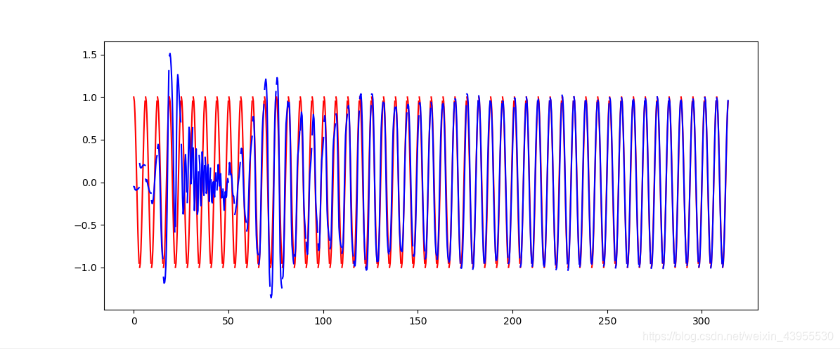
    plt.plot(steps, y_np.flatten(), 'r-')
    plt.plot(steps, prediction.data.numpy().flatten(), 'b-')
    plt.draw(); plt.pause(0.05)

plt.ioff()
plt.show()