点击上方“AI公园”，关注公众号，选择加“星标“或“置顶”

作者：Barış KaramanFollow

编译：ronghuaiyang

正文共：7785 字 13 图

预计阅读时间：23 分钟

导读

当我们流失用户进行了预测之后，为了留住这些可能会流失的客户，我们需要采取一些措施，我们希望了解客户未来一段时间内的行为，然后采取相应的行动。

前文回顾：

用机器学习来提升你的用户增长：第一步，了解你的目标

用机器学习来提升你的用户增长：第二步，客户分群

用机器学习来提升你的用户增长：第三步，预测客户的终生价值

用机器学习来提升你的用户增长：第四步，客户流失预测

第五部分: 预测下一个购买日

我们在数据驱动增长系列中解释的大多数行为背后都有相同的心态：

在客户期望(如LTV预测)之前，以客户想要的方式对待他们，并在糟糕的事情发生之前采取行动(如客户流失)。

预测分析对我们很有帮助。其中一个用途是预测客户的下一个购买日。如果你知道客户是否可能在7天内再次购买，该怎么办？

我们可以在此基础上建立我们的战略，并提出许多行动，如：

• 不要再给促销优惠给这个客户，因为他/她肯定会进行购买

• 如果在预测的时间窗口内没有购买的话，使用营销的方式推动客户(或者把做预测的家伙给炒了)

在本文中，我们将使用在线零售数据集，并遵循以下步骤：

• 数据整理(创建前一次/下一次数据集并计算购买日时间差)

• 特征工程

• 选择机器学习模型

• 多分类模型

• 超参数调优

数据整理

让我们从导入数据开始，做初步的数据工作：

#import libraries
from datetime import datetime, timedelta,date
import pandas as pd
%matplotlib inline
from sklearn.metrics import classification_report,confusion_matrix
import matplotlib.pyplot as plt
import numpy as np
import seaborn as sns
from __future__ import division
from sklearn.cluster import KMeans

#do not show warnings
import warnings
warnings.filterwarnings("ignore")

#import plotly for visualization
import plotly.plotly as py
import plotly.offline as pyoff
import plotly.graph_objs as go

#import machine learning related libraries
from sklearn.svm import SVC
from sklearn.multioutput import MultiOutputClassifier
from sklearn.ensemble import GradientBoostingClassifier
from sklearn.tree import DecisionTreeClassifier
from sklearn.neighbors import KNeighborsClassifier
from sklearn.naive_bayes import GaussianNB
from sklearn.ensemble import RandomForestClassifier
from sklearn.linear_model import LogisticRegression
import xgboost as xgb
from sklearn.model_selection import KFold, cross_val_score, train_test_split

#initiate plotly
pyoff.init_notebook_mode()

#import the csv
tx_data = pd.read_csv('data.csv')

#print first 10 rows
tx_data.head(10)

#convert date field from string to datetime
tx_data['InvoiceDate'] = pd.to_datetime(tx_data['InvoiceDate'])

#create dataframe with uk data only
tx_uk = tx_data.query("Country=='United Kingdom'").reset_index(drop=True)

导入CSV文件以及数据字段转换

我们已经导入了CSV文件，将日期字段从字符串转换为DateTime类型，并过滤了除英国以外的其他国家。

为了建立我们的模型，我们把数据分成两部分：

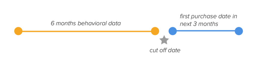
模型的数据结构

我们使用六个月的行为数据来预测顾客在未来三个月内的首次购买日期。如果没有购买，我们也会预测。我们假设我们的截止日期是2011年9月9日，并分割数据：

tx_6m = tx_uk[(tx_uk.InvoiceDate < date(2011,9,1)) & (tx_uk.InvoiceDate >= date(2011,3,1))].reset_index(drop=True)

tx_next = tx_uk[(tx_uk.InvoiceDate >= date(2011,9,1)) & (tx_uk.InvoiceDate < date(2011,12,1))].reset_index(drop=True)

tx_6m表示六个月的表现，我们使用tx_next来查找tx_6m中最后一次购买日期与tx_next中第一次购买日期之间的天数。

此外，我们将创建一个名为tx_user的dataframe，包含了预测模型需要使用的用户级特征集合：

tx_user = pd.DataFrame(tx_6m['CustomerID'].unique())
tx_user.columns = ['CustomerID']

通过使用tx_next中的数据，我们需要计算我们的label(截止日期前最后一次购买到截止日期后第一次购买之间的天数)：

#create a dataframe with customer id and first purchase date in tx_next
tx_next_first_purchase = tx_next.groupby('CustomerID').InvoiceDate.min().reset_index()
tx_next_first_purchase.columns = ['CustomerID','MinPurchaseDate']

#create a dataframe with customer id and last purchase date in tx_6m
tx_last_purchase = tx_6m.groupby('CustomerID').InvoiceDate.max().reset_index()
tx_last_purchase.columns = ['CustomerID','MaxPurchaseDate']

#merge two dataframes
tx_purchase_dates = pd.merge(tx_last_purchase,tx_next_first_purchase,on='CustomerID',how='left')

#calculate the time difference in days:
tx_purchase_dates['NextPurchaseDay'] = (tx_purchase_dates['MinPurchaseDate'] - tx_purchase_dates['MaxPurchaseDate']).dt.days

#merge with tx_user 
tx_user = pd.merge(tx_user, tx_purchase_dates[['CustomerID','NextPurchaseDay']],on='CustomerID',how='left')

#print tx_user
tx_user.head()

#fill NA values with 999
tx_user = tx_user.fillna(999)

现在，tx_user看起来像下面这样：

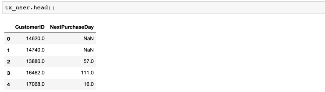
你很容易注意到，我们有NaN值，因为那些客户还没有进行任何购买。我们用999填入NaN以便稍后快速识别它们。

我们在这个dataframe中有客户id和相应的标签。我们加入特征集合，以构建我们的机器学习模型。

特征工程

对于这个项目，我们选择了我们的候选特征如下：

• RFM得分和聚类

• 最近三次购买之间的天数

• 以天为单位的购买时间差的平均值和标准偏差

在添加这些特征之后，我们需要通过应用get_dummies方法来处理类别特征。

RFM我们在第二篇文章中已经介绍过了。

让我们来关注一下如何添加接下来的两个特征。在这一部分中，我们将经常使用shift()方法。

首先，我们用客户ID和购买日期(而不是datetime)创建一个dataframe。然后我们将删除重复值，因为客户可以在一天内进行多次购买，这些时间的差为0。

#create a dataframe with CustomerID and Invoice Date
tx_day_order = tx_6m[['CustomerID','InvoiceDate']]
#convert Invoice Datetime to day
tx_day_order['InvoiceDay'] = tx_6m['InvoiceDate'].dt.date
tx_day_order = tx_day_order.sort_values(['CustomerID','InvoiceDate'])
#drop duplicates
tx_day_order = tx_day_order.drop_duplicates(subset=['CustomerID','InvoiceDay'],keep='first')

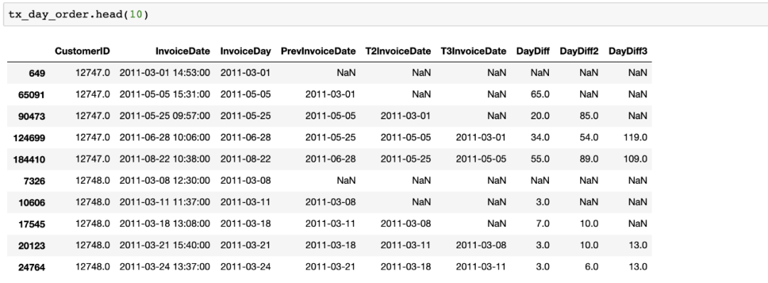
接下来，通过使用shift，我们创建了一个新的列，显示最近3次购买的日期，看看我们的dataframe是什么样子的：

#shifting last 3 purchase dates
tx_day_order['PrevInvoiceDate'] = tx_day_order.groupby('CustomerID')['InvoiceDay'].shift(1)
tx_day_order['T2InvoiceDate'] = tx_day_order.groupby('CustomerID')['InvoiceDay'].shift(2)
tx_day_order['T3InvoiceDate'] = tx_day_order.groupby('CustomerID')['InvoiceDay'].shift(3)

输出：

让我们开始计算每个购买日期的天数差：

tx_day_order['DayDiff'] = (tx_day_order['InvoiceDay'] - tx_day_order['PrevInvoiceDate']).dt.days
tx_day_order['DayDiff2'] = (tx_day_order['InvoiceDay'] - tx_day_order['T2InvoiceDate']).dt.days
tx_day_order['DayDiff3'] = (tx_day_order['InvoiceDay'] - tx_day_order['T3InvoiceDate']).dt.days

输出：

对于每个客户ID，我们使用.agg()方法来找出购买日的差的平均值和标准差：

tx_day_diff = tx_day_order.groupby('CustomerID').agg({'DayDiff': ['mean','std']}).reset_index()
tx_day_diff.columns = ['CustomerID', 'DayDiffMean','DayDiffStd']

现在我们要做一个艰难的决定。上面的计算对于有很多购买的客户是非常有用的。但是对于1-2次购买的人来说，情况就不一样了。例如，将一个在很短时间内只购买了两件商品的顾客标记为“频繁光顾”还为时过早。

我们只保留那些购买次数>3的客户：

tx_day_order_last = tx_day_order.drop_duplicates(subset=['CustomerID'],keep='last')

最后，我们删除NA值，合并新的dataframes与tx_user，并应用.get_dummies()转换类别值：

tx_day_order_last = tx_day_order_last.dropna()
tx_day_order_last = pd.merge(tx_day_order_last, tx_day_diff, on='CustomerID')
tx_user = pd.merge(tx_user, tx_day_order_last[['CustomerID','DayDiff','DayDiff2','DayDiff3','DayDiffMean','DayDiffStd']], on='CustomerID')
#create tx_class as a copy of tx_user before applying get_dummies
tx_class = tx_user.copy()
tx_class = pd.get_dummies(tx_class)

我们的特征集合已经为构建好了，可以开始做分类模型了。但是有很多不同的模型，我们应该使用哪一个呢？

选择一个机器学习模型

在开始选择模型之前，我们需要采取两个行动。首先，我们需要标识标签中的分类。一般来说，用百分位数看可以。我们使用.describe()方法在NextPurchaseDay中查看它们：

对于统计数据和业务需求来说，确定边界都是一个问题。首先，它应该要有意义，另外需要很容易采取行动和沟通。考虑到这两个，我们分为三个类：

• 0-20: 0-20天内购买的客户 — 类名:2

• 21-49: 21-49天内购买的客户 —  类名:1

• ≥50：在50天内购买的客户 — 类名:0

tx_class['NextPurchaseDayRange'] = 2
tx_class.loc[tx_class.NextPurchaseDay>20,'NextPurchaseDayRange'] = 1
tx_class.loc[tx_class.NextPurchaseDay>50,'NextPurchaseDayRange'] = 0

最后一步是查看我们的特征和标签之间的相关性。相关矩阵是最简洁的表示方法之一：

corr = tx_class[tx_class.columns].corr()
plt.figure(figsize = (30,20))
sns.heatmap(corr, annot = True, linewidths=0.2, fmt=".2f")

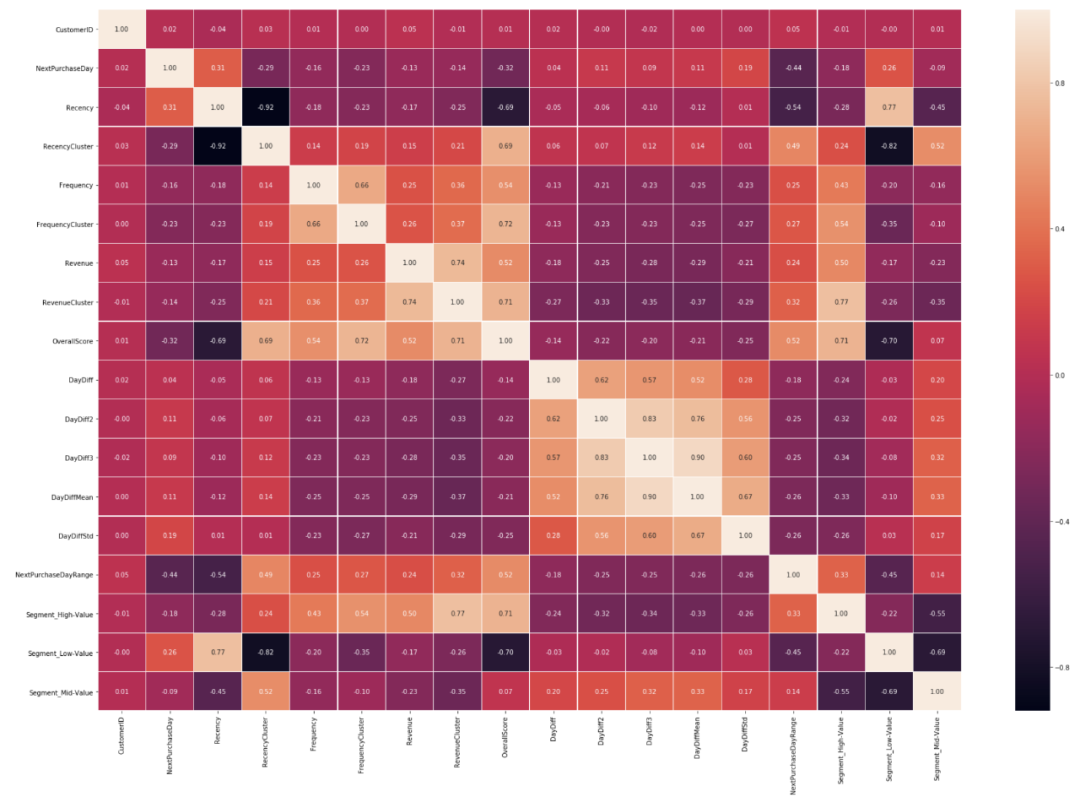
Overall Score的正相关系数最高(0.45)，Recency的负相关系数最高(-0.54)。

对于这个特殊的问题，我们希望使用精度最高的模型。我们分别进行训练和测试，测试不同模型的准确性：

#train & test split
tx_class = tx_class.drop('NextPurchaseDay',axis=1)
X, y = tx_class.drop('NextPurchaseDayRange',axis=1), tx_class.NextPurchaseDayRange
X_train, X_test, y_train, y_test = train_test_split(X, y, test_size=0.2, random_state=44)

#create an array of models
models = []
models.append(("LR",LogisticRegression()))
models.append(("NB",GaussianNB()))
models.append(("RF",RandomForestClassifier()))
models.append(("SVC",SVC()))
models.append(("Dtree",DecisionTreeClassifier()))
models.append(("XGB",xgb.XGBClassifier()))
models.append(("KNN",KNeighborsClassifier()))

#measure the accuracy 
for name,model in models:
    kfold = KFold(n_splits=2, random_state=22)
    cv_result = cross_val_score(model,X_train,y_train, cv = kfold,scoring = "accuracy")
    print(name, cv_result)

选择准确率最高的机器学习模型

每个模型的准确率：

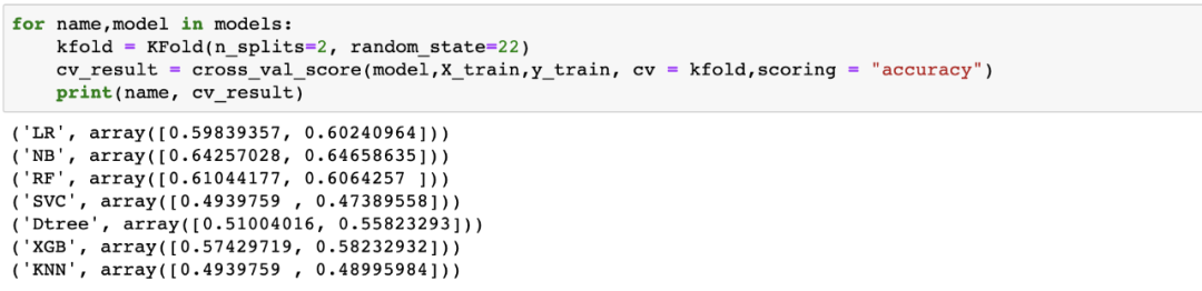
从这个结果可以看出，朴素贝叶斯是最优的一种算法(正确率约为64%)。但在那之前，让我们看看我们到底做了什么。我们在机器学习中应用了一个基本的概念，那就是交叉验证。

我们如何确保机器学习模型在不同数据集上的稳定性？另外，如果在我们选择的测试集中有噪声会怎样？

交叉验证是一种衡量方法。它通过选择不同的测试集来得到模型的分数。如果偏差很小，则意味着模型是稳定的。在我们的例子中，分数之间的偏差是可以接受的(除了决策树分类器)。

通常，我们应该使用朴素贝叶斯。但是对于这个例子，让我们继续使用XGBoost来展示如何使用一些高级技术来改进现有的模型。

多分类模型

要构建我们的模型，我们将遵循前几篇文章中的步骤。但是为了进一步改进它，我们将执行超参数调优。

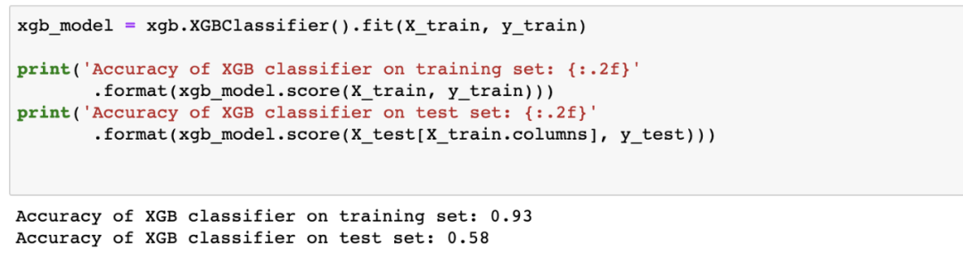
通过编程，我们将找出我们的模型的最佳参数，使其提供最佳的准确性。让我们先从我们的模型代码开始：

xgb_model = xgb.XGBClassifier().fit(X_train, y_train)print('Accuracy of XGB classifier on training set: {:.2f}'
       .format(xgb_model.score(X_train, y_train)))
print('Accuracy of XGB classifier on test set: {:.2f}'
       .format(xgb_model.score(X_test[X_train.columns], y_test)))

在这个版本中，我们测试集的准确率为58%：

XGBClassifier有很多参数。你可以在这里找到这些参数的列表。对于本例，我们选择max_depth和min_child_weight.

下面的代码将为这些参数生成最佳值：

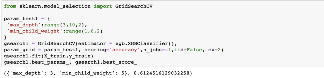
该算法表示，max_depth和min_child_weight的最佳值分别为3和5。看看它是如何提高准确性的：

我们的分数从58%上升到了62%。这是一个很大的进步。

知道下一个购买日也是预测销售的好指标。我们将在下一部分中深入探讨这个主题。

—END—

英文原文：https://towardsdatascience.com/predicting-next-purchase-day-15fae5548027

请长按或扫描二维码关注本公众号

喜欢的话，请给我个好看吧！