连享会-文本分析与爬虫专题研讨班
诚邀助教:连享会-文本分析与爬虫专题

之前的教程中我们介绍了如何使用 ggplot2 + sf 绘制中国地图,使用这种方法我们需要准备 shp 数据,这个数据似乎网上都比较抠,不好找,好数据都收费!这篇教程中我们介绍一种新的数据——GEOJSON(这种数据网上一大堆),使用该数据的最好方法就是先把 GEOJSON 对象转换为 sf 对象然后再用我们的老方法绘制地图。除此之外,本文还介绍了如何获取 GEOJSON 数据、如何在交互式图表中使用 GEOJSON 数据。
使用 ggplot2 + sf + geojson 数据绘制地图
首先,第一步,获取 GEOJSON 数据,获取源1: https://gallery.echartsjs.com/editor.html?c=xr1IEt3r4Q ,这样的:
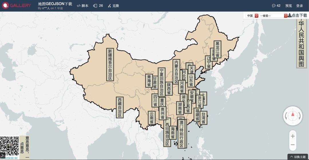
根据自己的需要下载即可,下载后可以得到 json 文件,例如我们下载一份
全国.json
数据,然后用这个数据绘制地图。
第一步:把该 json 数据读入 R 中,有两种方法,方法一:
注意:使用直接下载得到的 json 文件运行上面的程序是会出错的,可以手动打开 json 文件在文件的末尾空一行。
# install.packages("geojsonsf")library(geojsonsf)chinasf1 % paste0(collapse = "") %>% geojsonsf::geojson_sf()第二种方法:
library(sf)chinasf2 ## Reading layer `全国' from data source `/Users/czx/Desktop/使用GEOJSON数据绘制地图/全国.json' using driver `GeoJSON'## Simple feature collection with 34 features and 8 fields## geometry type: MULTIPOLYGON## dimension: XY## bbox: xmin: 73.50235 ymin: 3.840015 xmax: 135.0957 ymax: 53.56327## epsg (SRID): 4326## proj4string: +proj=longlat +datum=WGS84 +no_defs可以用下面的方法比较两种读取方法的速度:
# 速度比较library(microbenchmark)microbenchmark( geojson_sf = { readLines("全国.json") %>% paste0(collapse = "") %>% geojsonsf::geojson_sf() }, sf = { sf::st_read("全国.json", quiet = T) }, times = 5)## Unit: milliseconds## expr min lq mean median uq max neval cld## geojson_sf 19.86315 20.71012 22.29798 23.36813 23.75352 23.79499 5 a ## sf 70.77053 71.32985 74.72381 72.39345 74.20421 84.92100 5 b
可以看出,
sf::st_read
虽然读取方便,但是比
geojsonsf::geojson_sf
慢。
chinasf % paste0(collapse = "") %>% geojsonsf::geojson_sf()
chinasf
是个 sf 对象:
class(chinasf)## [1] "sf" "data.frame"glimpse(chinasf)## Observations: 34## Variables: 9## $ adcode 110000, 120000, 130000, 140000, 150000, 210000, 22000…## $ center "[116.405285,39.904989]", "[117.190182,39.125596]", "…## $ name "北京市", "天津市", "河北省", "山西省", "内蒙古自治区", "辽宁省", "吉林省", "…## $ centroid "[116.419889,40.189911]", "[117.347019,39.28803]", NA…## $ childrenNum 16, 16, 11, 11, 12, 14, 9, 13, 16, 13, 11, 16, 9, 11,…## $ level "province", "province", "province", "province", "prov…## $ subFeatureIndex 0, 1, 2, 3, 4, 5, 6, 7, 8, 9, 10, 11, 12, 13, 14, 15,…## $ acroutes "[100000]", "[100000]", "[100000]", "[100000]", "[100…## $ geometry MULTIPOLYGON (((116.8121 39..., MULTIPOL…第二步,我们生成一个虚拟的变量 pop:
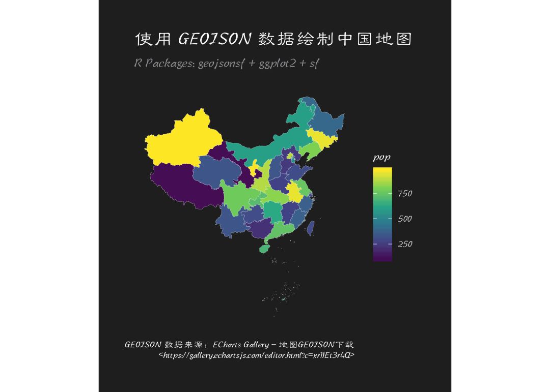
chinasf$pop 然后我们使用之前介绍的 ggplot2 + sf 绘制一幅地图:
library(ggplot2)cnfont = "STLibianSC-Regular"enfont = "CascadiaCode-Regular"ggplot() + geom_sf(data = chinasf, aes(geometry = geometry, fill = pop), size = 0.05, color = "white") + coord_sf(crs = "+proj=laea +lat_0=23 +lon_0=113 +x_0=4321000 +y_0=3210000 +ellps=GRS80 +units=m +no_defs") + scale_fill_viridis_c() + theme_modern_rc(base_family = cnfont, subtitle_family = cnfont, caption_family = cnfont) + worldtilegrid::theme_enhance_wtg() + labs(title = "使用 GEOJSON 数据绘制中国地图", subtitle = "R Packages: geojsonsf + ggplot2 + sf", caption = "GEOJSON 数据来源:ECharts Gallery - 地图GEOJSON下载\n")
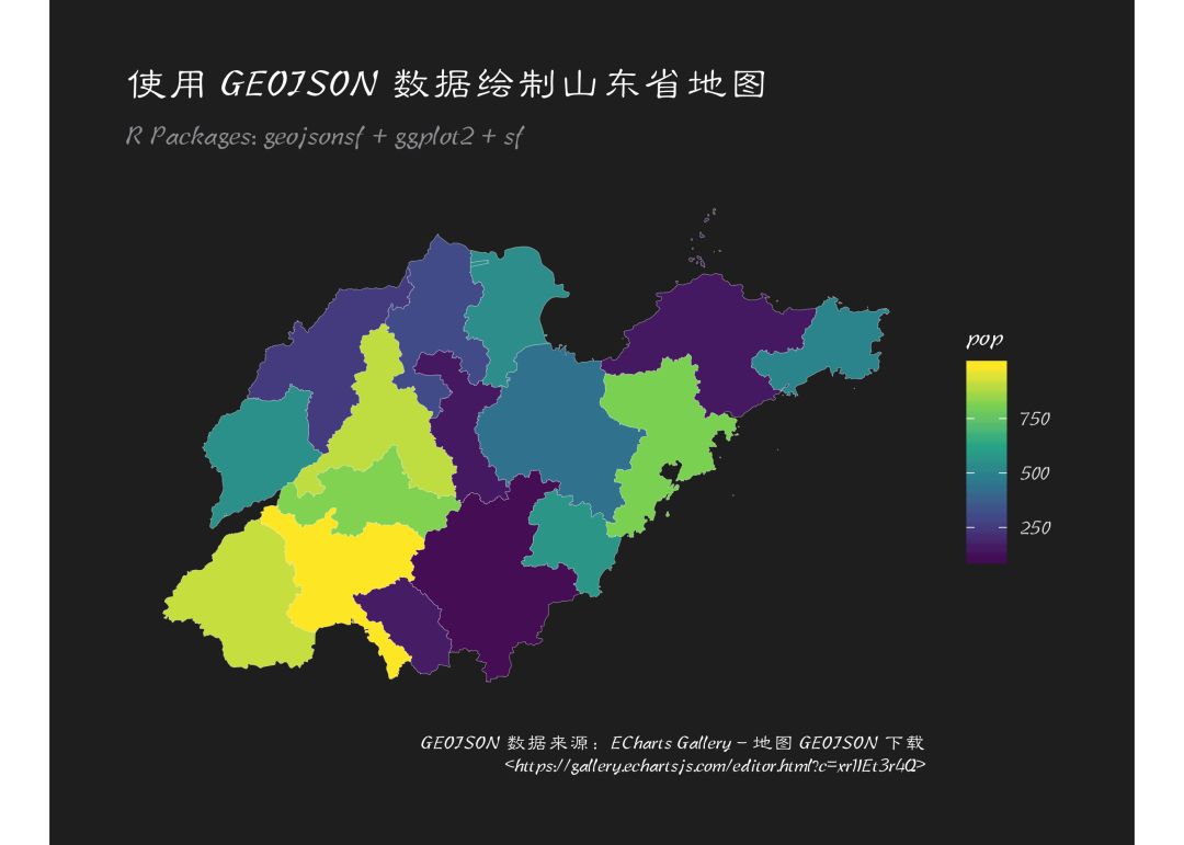
绘制山东地图
同样的方法,我们下载一个山东省的数据然后绘制山东地图:
sdsf % paste0(collapse = "") %>% geojsonsf::geojson_sf()sdsf$pop ggplot() + geom_sf(data = sdsf, aes(geometry = geometry, fill = pop), size = 0.05, color = "white") + coord_sf(crs = "+proj=laea +lat_0=23 +lon_0=113 +x_0=4321000 +y_0=3210000 +ellps=GRS80 +units=m +no_defs") + scale_fill_viridis_c() + theme_modern_rc(base_family = cnfont, subtitle_family = cnfont, caption_family = cnfont) + worldtilegrid::theme_enhance_wtg() + labs(title = "使用 GEOJSON 数据绘制山东省地图", subtitle = "R Packages: geojsonsf + ggplot2 + sf", caption = "GEOJSON 数据来源:ECharts Gallery - 地图 GEOJSON 下载\n")
其它省市的地图绘制方法相同,可以自己尝试下!
使用 GEOJSON 绘制交互式地图
绘制交互式地图的包蛮多的,我这里演示 highcharter、echarts4r 和 leaflet。
使用 highcharter + geojson 绘制中国地图
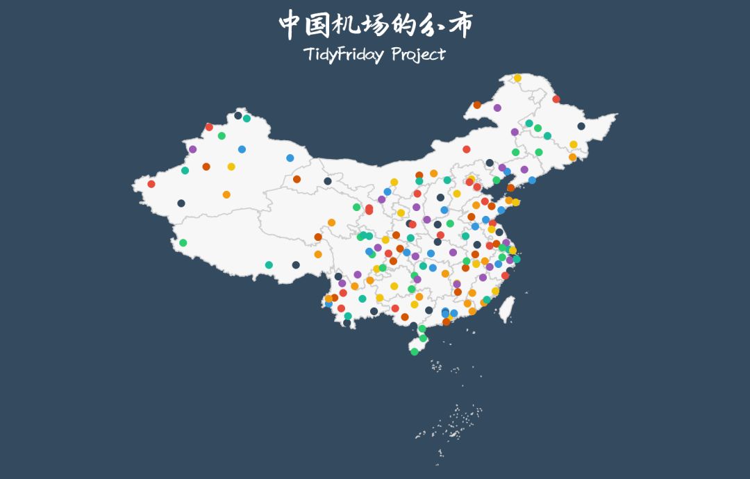
这里我绘制了一幅中国机场分布的地图:
# install.packages("geojsonio")# install.packages("geojsonlint")library(readr)library(geojsonio)library(highcharter)library(jsonlite)cngeojson simplifyVector = F) %>% as.json()# global_airports.csv: 全球机场的分布airports % dplyr::filter(country == "China")airp_geojson airports, lat = "latitude", lon = "longitude")highchart(type = "map") %>% hc_add_series(mapData = cngeojson, showInLegend = F) %>% hc_add_series(data = airp_geojson, type = "mappoint", dataLabels = list( enabled = F ), colorByPoint = T) %>% hc_tooltip(shared = F, formatter = JS( "function(){ return '' + this.point.name + ''; }" )) %>% hc_title(text = "中国机场的分布", style = list(fontFamily = "SentyZHAO", fontSize = "32px")) %>% hc_legend(enabled = F) %>% hc_subtitle(text = "TidyFriday Project", style = list(fontFamily = "SentyZHAO", fontSize = "20px", color = "#FFFFFF")) %>% hc_add_theme(hc_theme_flatdark())
使用 echarts4r + geojson 绘制中国地图
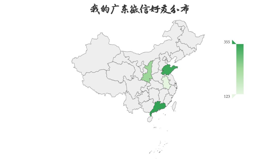
这里我使用的是手动随机生成的数据:
library(echarts4r)library(tibble)json df ~prov, ~pop, "安徽省", 123, "广东省", 355, "山东省", 343, "陕西省", 243)df %>% e_charts(prov) %>% e_map_register("全国", json) %>% e_map(pop, map = "全国") %>% e_visual_map(pop, color = c(rev(brewer.pal(3, "Greens"))), left = '80%', top = '20%') %>% e_title("我的广东微信好友分布", textStyle = list("fontSize" = 30, "fontFamily" = "SentyZHAO"), textAlign = "middle", left = "50%")
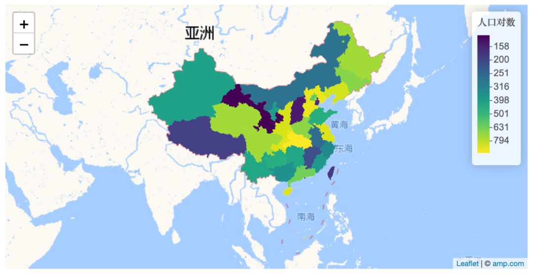
使用 leaflet + geojson 绘制中国地图
这里我再次演示了如何为 leaflet 地图添加标题(这个标题在 RMarkdown 文档里似乎无法显示),这里我使用的是 leafletCN 包提供的高德地图作为底图:
library(leaflet)library(leafletCN)library(htmltools)library(manipulateWidget)# 为 leaflet 地图添加标题(这个标题在 RMarkdown 文档里似乎无法显示)tag.map.title .leaflet-control.map-title { transform: translate(-50%,20%); position: fixed !important; left: 50%; text-align: center; padding-left: 10px; padding-right: 10px; background-color:transparent; font-weight: bold; font-size: 28px; font-family: SentyZHAO; }"))title tag.map.title, HTML("中国地图"))cn pal cn$pop leaflet(cn) %>% amap() %>% addPolygons(stroke = FALSE, smoothFactor = 0.3, fillOpacity = 1, fillColor = ~pal(log10(pop)), label = ~paste0(name, ": ", formatC(pop, big.mark = ","))) %>% addLegend(pal = pal, values = ~log10(pop), opacity = 1.0, labFormat = labelFormat(transform = function(x) round(10^x)), title = "人口对数") %>% addControl(title, position = "topleft", className = "map-title") %>% combineWidgets(byrow = TRUE, ncol = 1, width = "100%", height = "400px")
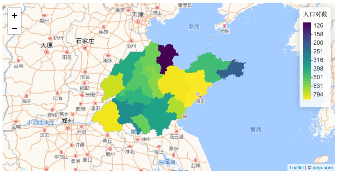
再绘制一幅山东地图:
sd title tag.map.title, HTML("山东地图"))sd$pop leaflet(sd) %>% amap() %>% addPolygons(stroke = FALSE, smoothFactor = 0.3, fillOpacity = 1, fillColor = ~pal(log10(pop)), label = ~paste0(name, ": ", formatC(pop, big.mark = ","))) %>% addLegend(pal = pal, values = ~log10(pop), opacity = 1.0, labFormat = labelFormat(transform = function(x) round(10^x)), title = "人口对数") %>% addControl(title, position = "topleft", className = "map-title") %>% combineWidgets(byrow = TRUE, ncol = 1, width = "100%", height = "400px")
还可以再深入一下,绘制威海的地图:
wh title tag.map.title, HTML("威海地图"))wh$pop leaflet(wh) %>% amap() %>% addPolygons(stroke = FALSE, smoothFactor = 0.3, fillOpacity = 0.5, fillColor = ~pal(log10(pop)), label = ~paste0(name, ": ", formatC(pop, big.mark = ","))) %>% addLegend(pal = pal, values = ~log10(pop), opacity = 0.5, labFormat = labelFormat(transform = function(x) round(10^x)), title = "人口对数") %>% addControl(title, position = "topleft", className = "map-title") %>% combineWidgets(byrow = TRUE, ncol = 1, width = "100%", height = "400px")
其它获取 geojson 数据的地址:
1.https://gallery.echartsjs.com/editor.html?c=xBkM-72arM2.https://github.com/ufoe/d3js-geojson
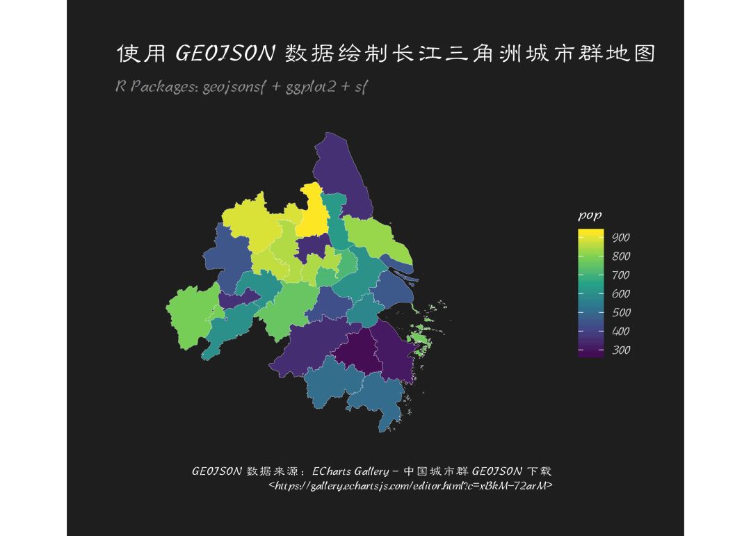
绘制长江三角洲城市群地图
数据来源:https://gallery.echartsjs.com/editor.html?c=xBkM-72arM
library(sf)csjsf ## Reading layer `长江三角洲城市群' from data source `/Users/czx/Desktop/使用GEOJSON数据绘制地图/长江三角洲城市群.json' using driver `GeoJSON'## Simple feature collection with 26 features and 7 fields## geometry type: MULTIPOLYGON## dimension: XY## bbox: xmin: 115.7623 ymin: 28.01226 xmax: 122.9462 ymax: 34.48554## epsg (SRID): 4326## proj4string: +proj=longlat +datum=WGS84 +no_defscsjsf$pop ggplot() + geom_sf(data = csjsf, aes(geometry = geometry, fill = pop), size = 0.05, color = "white") + coord_sf(crs = "+proj=laea +lat_0=23 +lon_0=113 +x_0=4321000 +y_0=3210000 +ellps=GRS80 +units=m +no_defs") + scale_fill_viridis_c() + theme_modern_rc(base_family = cnfont, subtitle_family = cnfont, caption_family = cnfont) + worldtilegrid::theme_enhance_wtg() + labs(title = "使用 GEOJSON 数据绘制长江三角洲城市群地图", subtitle = "R Packages: geojsonsf + ggplot2 + sf", caption = "GEOJSON 数据来源:ECharts Gallery - 中国城市群 GEOJSON 下载\n") + coord_sf(xlim = c(125, 115))
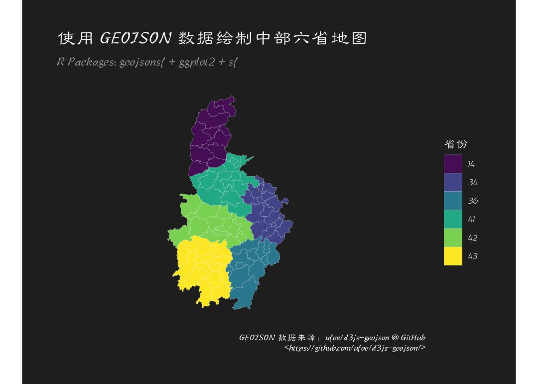
使用多个 GEOJSON 数据绘制组合地图:绘制中部六省的地图
这里我演示了如何使用 6 个 json 数据文件绘制中部六省的地图:
数据来源:https://github.com/ufoe/d3js-geojson
# 批量下载数据:# for(i in c(14, 34, 36, 41, 42, 43)){# download.file(paste0('https://github.com/ufoe/d3js-geojson/raw/master/china/geometryProvince/', i, '.json'), paste0(i, '.json'))# }df ## Reading layer `14' from data source `/Users/czx/Desktop/使用GEOJSON数据绘制地图/14.json' using driver `GeoJSON'## Simple feature collection with 11 features and 4 fields## geometry type: POLYGON## dimension: XY## bbox: xmin: 110.2258 ymin: 34.585 xmax: 114.5654 ymax: 40.7428## epsg (SRID): 4326## proj4string: +proj=longlat +datum=WGS84 +no_defsfor(i in c(34, 36, 41, 42, 43)){ df }## Reading layer `34' from data source `/Users/czx/Desktop/使用GEOJSON数据绘制地图/34.json' using driver `GeoJSON'## Simple feature collection with 17 features and 4 fields## geometry type: MULTIPOLYGON## dimension: XY## bbox: xmin: 114.884 ymin: 29.3939 xmax: 119.6521 ymax: 34.6509## epsg (SRID): 4326## proj4string: +proj=longlat +datum=WGS84 +no_defs## Reading layer `36' from data source `/Users/czx/Desktop/使用GEOJSON数据绘制地图/36.json' using driver `GeoJSON'## Simple feature collection with 11 features and 4 fields## geometry type: POLYGON## dimension: XY## bbox: xmin: 113.5767 ymin: 24.4885 xmax: 118.4875 ymax: 30.0751## epsg (SRID): 4326## proj4string: +proj=longlat +datum=WGS84 +no_defs## Reading layer `41' from data source `/Users/czx/Desktop/使用GEOJSON数据绘制地图/41.json' using driver `GeoJSON'## Simple feature collection with 17 features and 4 fields## geometry type: POLYGON## dimension: XY## bbox: xmin: 110.3577 ymin: 31.3824 xmax: 116.6528 ymax: 36.3647## epsg (SRID): 4326## proj4string: +proj=longlat +datum=WGS84 +no_defs## Reading layer `42' from data source `/Users/czx/Desktop/使用GEOJSON数据绘制地图/42.json' using driver `GeoJSON'## Simple feature collection with 17 features and 4 fields## geometry type: MULTIPOLYGON## dimension: XY## bbox: xmin: 108.3691 ymin: 29.0314 xmax: 116.1365 ymax: 33.2721## epsg (SRID): 4326## proj4string: +proj=longlat +datum=WGS84 +no_defs## Reading layer `43' from data source `/Users/czx/Desktop/使用GEOJSON数据绘制地图/43.json' using driver `GeoJSON'## Simple feature collection with 14 features and 4 fields## geometry type: POLYGON## dimension: XY## bbox: xmin: 108.7866 ymin: 24.6368 xmax: 114.2578 ymax: 30.1245## epsg (SRID): 4326## proj4string: +proj=longlat +datum=WGS84 +no_defs# 生成省份变量: id 的前两位df$prov ggplot() + geom_sf(data = df, aes(geometry = geometry, fill = factor(prov)), size = 0.05, color = "white") + coord_sf(crs = "+proj=laea +lat_0=23 +lon_0=113 +x_0=4321000 +y_0=3210000 +ellps=GRS80 +units=m +no_defs") + scale_fill_viridis_d(name = "省份") + theme_modern_rc(base_family = cnfont, subtitle_family = cnfont, caption_family = cnfont) + worldtilegrid::theme_enhance_wtg() + labs(title = "使用 GEOJSON 数据绘制中部六省地图", subtitle = "R Packages: geojsonsf + ggplot2 + sf", caption = "GEOJSON 数据来源:ufoe/d3js-geojson @ GitHub\n") + coord_sf(xlim = c(130, 100))
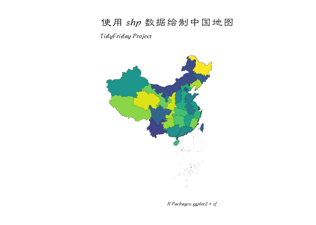
注意到这个合并数据集实际上也是将 geojson 数据先转化为 sf 数据框再合并的,所以我们之前每次绘制中国地图都用两个数据集实际上是可以只使用一个合并数据集的:
mapborder mapdata cndf names(cndf) cndf # 用这个数据画出来的地图是这样的:ggplot() + geom_sf(data = cndf, aes(geometry = geometry, fill = NAME), size = 0.05, color = "black") + scale_fill_viridis_d(name = "省份") + theme_ipsum(base_family = cnfont, subtitle_family = cnfont, caption_family = cnfont) + worldtilegrid::theme_enhance_wtg() + labs(title = "使用 shp 数据绘制中国地图", subtitle = "TidyFriday Project", caption = "R Packages: ggplot2 + sf") + guides(fill = "none")
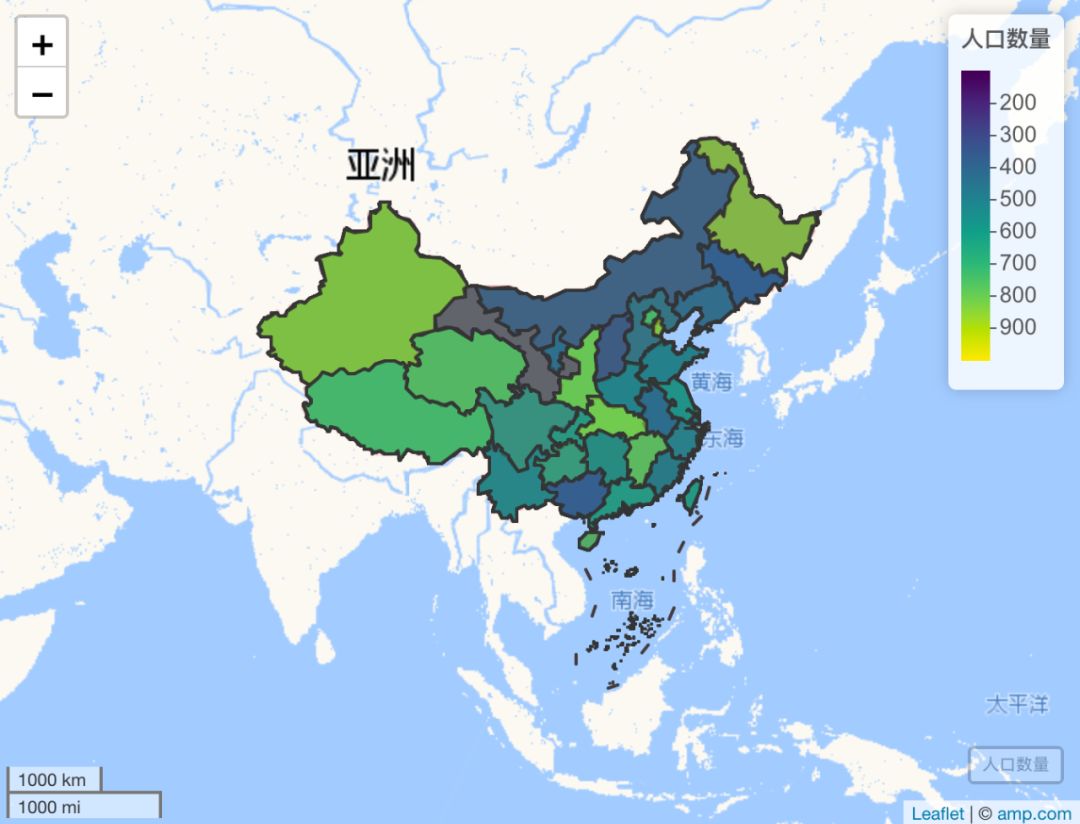
我们还可以将合并后的 sf 对象应用在 leaflet 地图上:
# install.packages("mapview")library(mapview)cndf$pop 1416, mapview(cndf, zcol = "pop", layer.name = "人口数量")
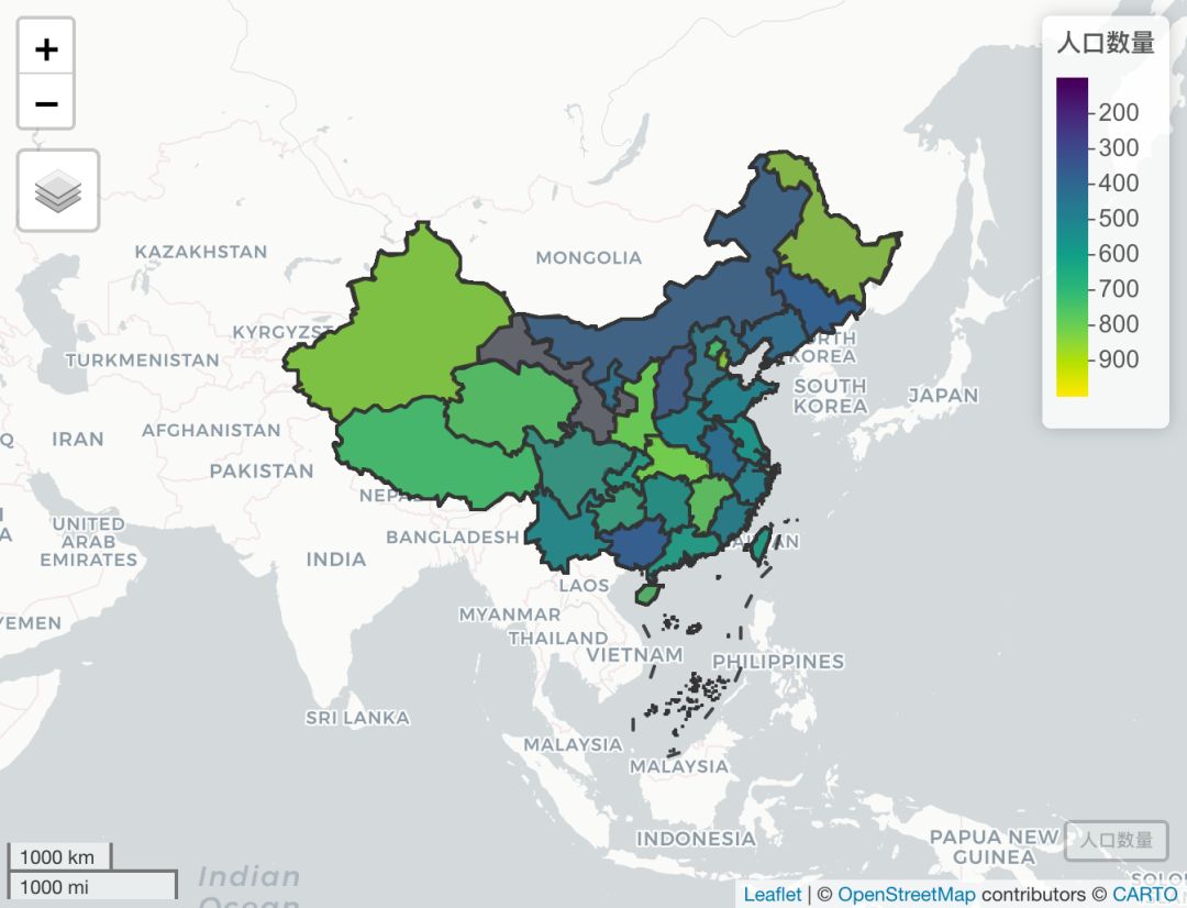
另外也可以使用高德地图作为底图:
leaflet(width = "100%", height = "400px") %>% amap() %>% mapview(cndf, zcol = "pop", layer.name = "人口数量", map = .)
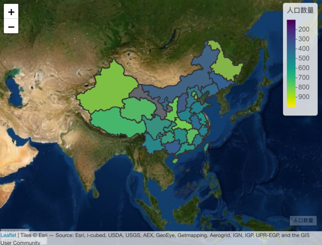
使用 Esri.WorldImagery 作为底图(卫星地图):
leaflet(width = "100%", height = "400px") %>% addProviderTiles("Esri.WorldImagery") %>% mapview(cndf, zcol = "pop", layer.name = "人口数量", map = .)
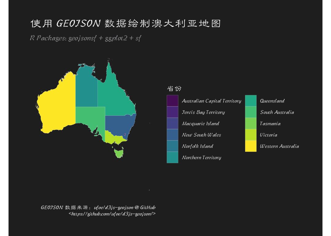
绘制外国地图
# 例如 澳大利亚 地图# download.file('https://github.com/ufoe/d3js-geojson/raw/master/Australia.json', 'Australia.json')Australia ## Reading layer `Australia' from data source `/Users/czx/Desktop/使用GEOJSON数据绘制地图/Australia.json' using driver `GeoJSON'## Simple feature collection with 11 features and 59 fields## geometry type: MULTIPOLYGON## dimension: XY## bbox: xmin: 112.9194 ymin: -54.75042 xmax: 159.1065 ymax: -9.240167## epsg (SRID): 4326## proj4string: +proj=longlat +datum=WGS84 +no_defsggplot() + geom_sf(data = Australia, aes(geometry = geometry, fill = name), size = 0.05, color = "white") + scale_fill_viridis_d(name = "省份") + theme_modern_rc(base_family = cnfont, subtitle_family = cnfont, caption_family = cnfont) + worldtilegrid::theme_enhance_wtg() + labs(title = "使用 GEOJSON 数据绘制澳大利亚地图", subtitle = "R Packages: geojsonsf + ggplot2 + sf", caption = "GEOJSON 数据来源:ufoe/d3js-geojson @ GitHub\n") + guides(fill = guide_legend(ncol = 2))
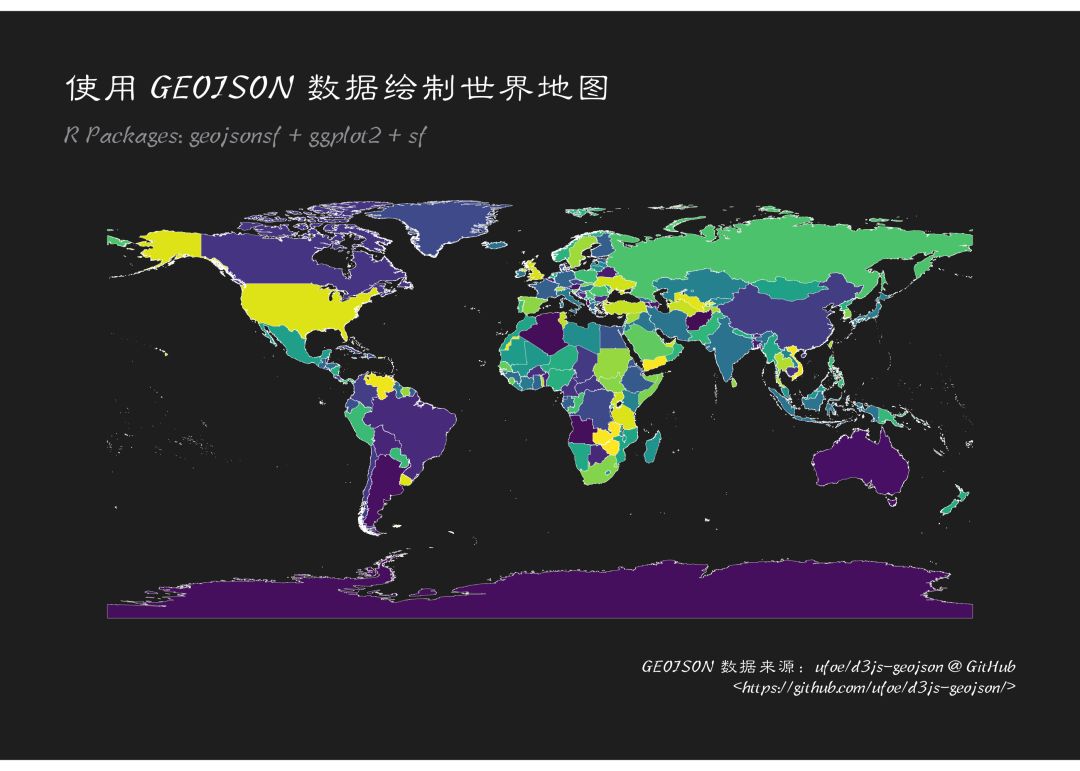
绘制世界地图
library(geojsonsf)library(sf)wdf ## Reading layer `world' from data source `/Users/czx/Desktop/使用GEOJSON数据绘制地图/world.json' using driver `GeoJSON'## Simple feature collection with 255 features and 65 fields## geometry type: MULTIPOLYGON## dimension: XY## bbox: xmin: -180 ymin: -90 xmax: 180 ymax: 83.6341## epsg (SRID): 4326## proj4string: +proj=longlat +datum=WGS84 +no_defs# coord_sf: crs: https://geocompr.robinlovelace.net/reproj-geoggplot() + geom_sf(data = wdf, aes(geometry = geometry, fill = SOVEREIGNT), size = 0.05, color = "white") + coord_sf(crs = "+proj=longlat") + scale_fill_viridis_d() + theme_modern_rc(base_family = cnfont, subtitle_family = cnfont, caption_family = cnfont) + labs(title = "使用 GEOJSON 数据绘制世界地图", subtitle = "R Packages: geojsonsf + ggplot2 + sf", caption = "GEOJSON 数据来源:ufoe/d3js-geojson @ GitHub\n") + theme_modern_rc(base_family = cnfont, subtitle_family = cnfont, caption_family = cnfont) + worldtilegrid::theme_enhance_wtg() + theme(legend.position = "none")
更改投影
最后我们再稍微讨论一下投影参数,这个东西比较复杂,我找了个文献放在附件里供大家参考,我这里演示常用的一些投影坐标系。
首先使用
st_crs(wdf)$proj4string
可以查看 sf 对象预置的 crs(coordinate reference systems):
st_crs(wdf)$proj4string## [1] "+proj=longlat +datum=WGS84 +no_defs"
coord_sf(crs = “+proj=longlat”): 这种坐标系是经线相互平行的:
p geom_sf(data = wdf, aes(geometry = geometry, fill = SOVEREIGNT), size = 0.05, color = "white") + scale_fill_viridis_d() + theme_modern_rc(base_family = cnfont, subtitle_family = cnfont, caption_family = cnfont) + labs(title = "使用 GEOJSON 数据绘制世界地图", subtitle = "R Packages: geojsonsf + ggplot2 + sf", caption = "GEOJSON 数据来源:ufoe/d3js-geojson @ GitHub\n") + theme_modern_rc(base_family = cnfont, subtitle_family = cnfont, caption_family = cnfont) + theme(legend.position = "none")p + coord_sf(crs = "+proj=longlat") + labs(title = 'coord_sf(crs = "+proj=longlat")')

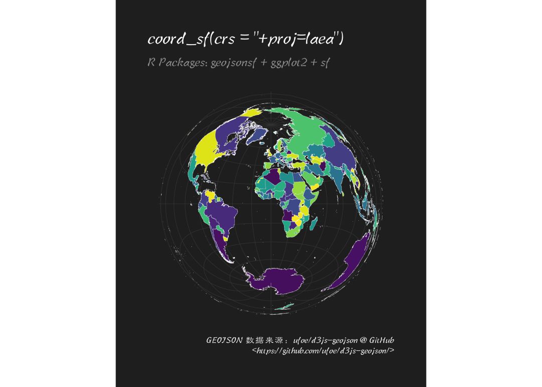
coord_sf(crs = “+proj=laea”): 球形地图
p + coord_sf(crs = "+proj=laea") + labs(title = 'coord_sf(crs = "+proj=laea")')
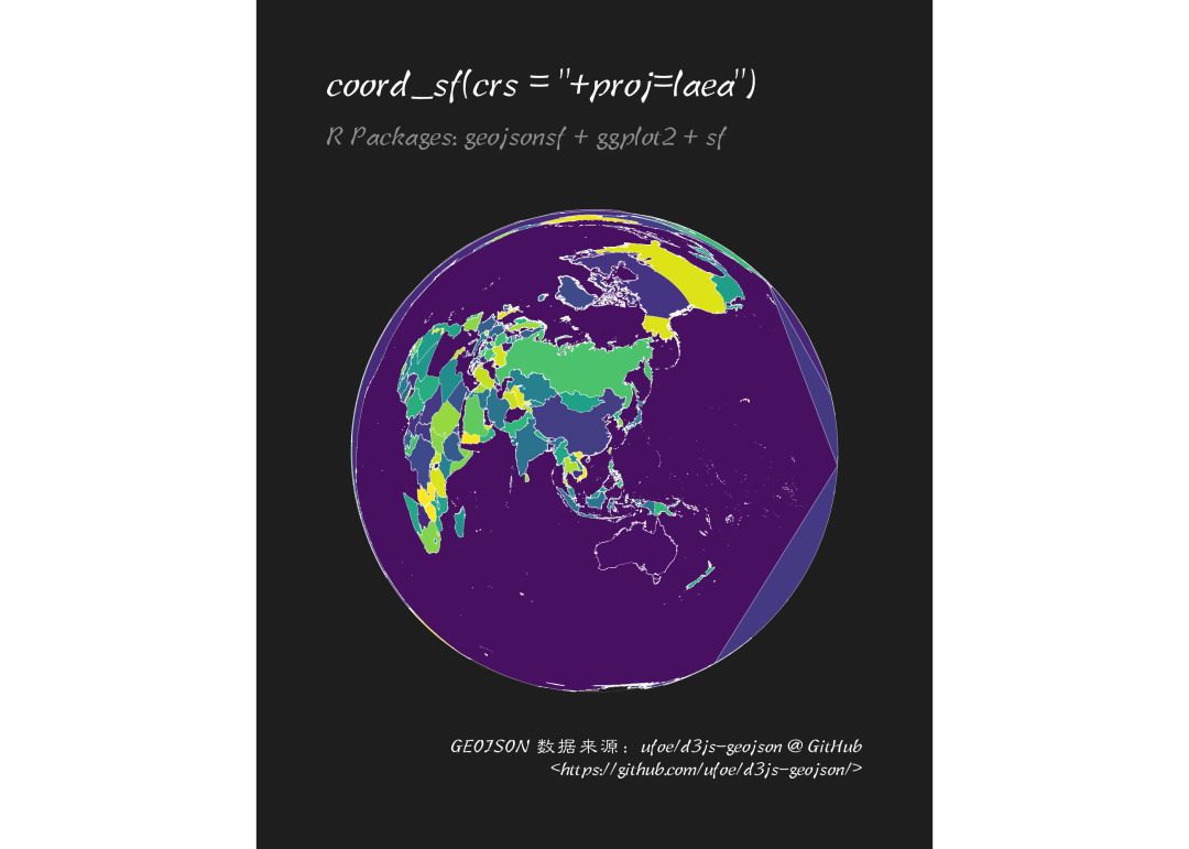
选择中心,例如暨南大学的经纬度为:(113, 23),以此为中心绘制地图:
p + coord_sf(crs = "+proj=laea +lon_0=113 +lat_0=23 +datum=WGS84 +no_defs") + labs(title = 'coord_sf(crs = "+proj=laea")')
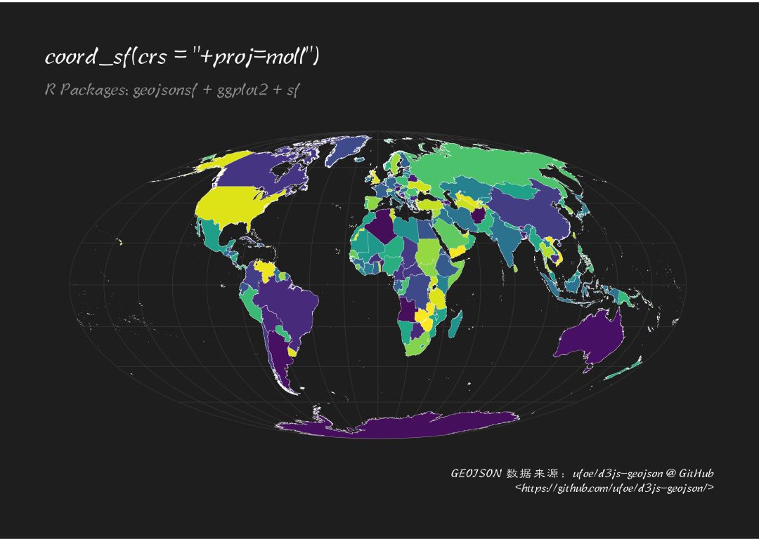
coord_sf(crs = “+proj=moll”): Mollweide 投影
p + coord_sf(crs = "+proj=moll") + labs(title = 'coord_sf(crs = "+proj=moll")')
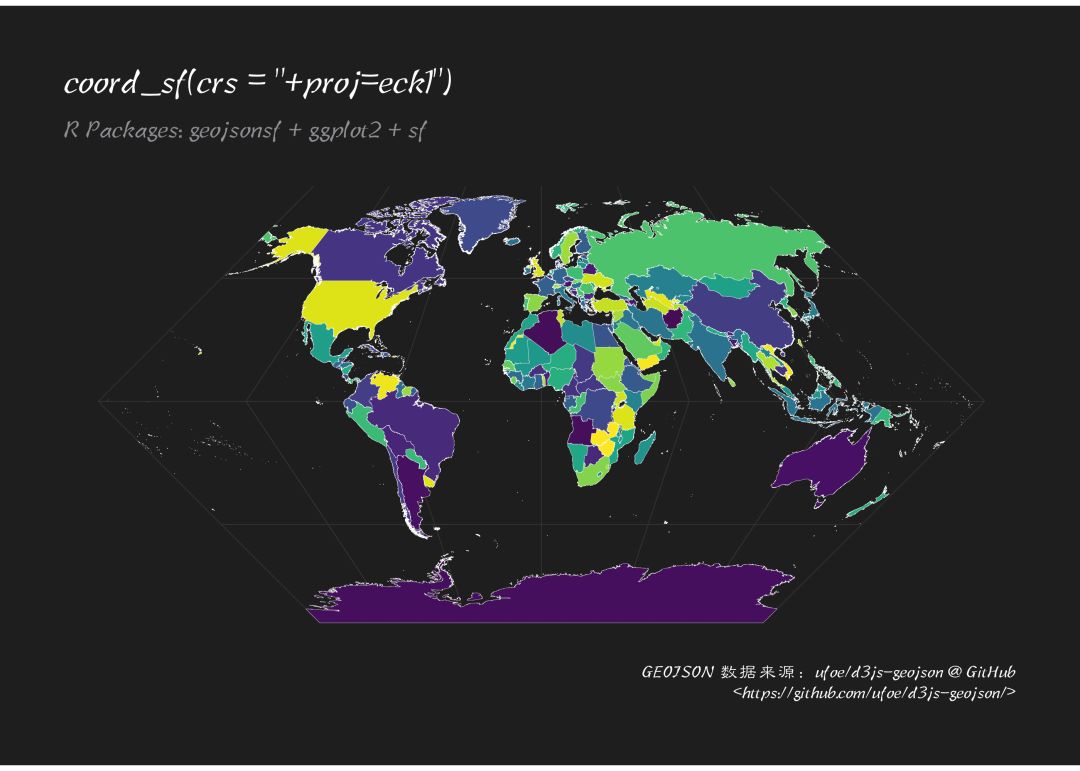
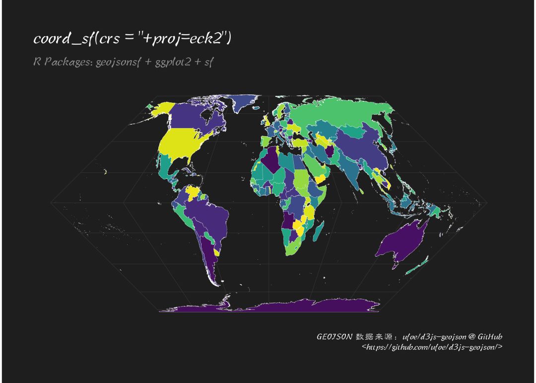
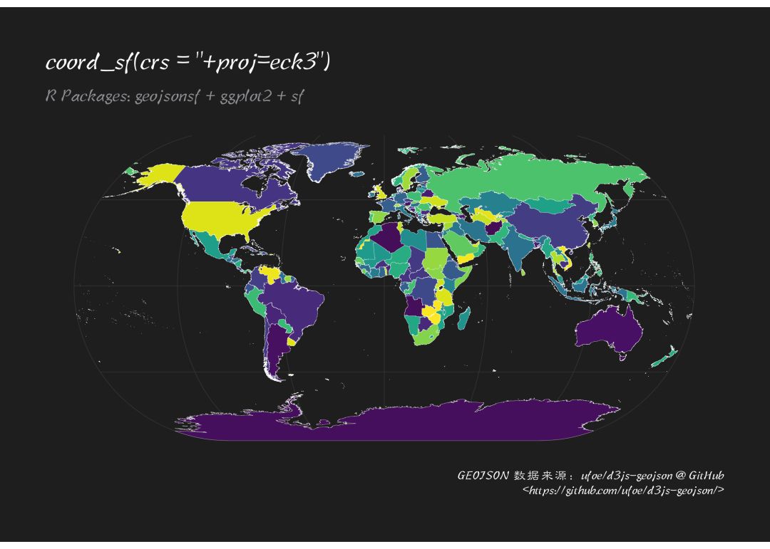
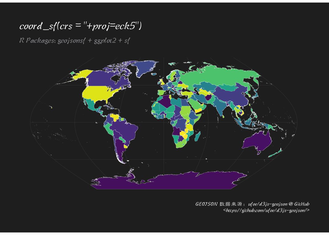
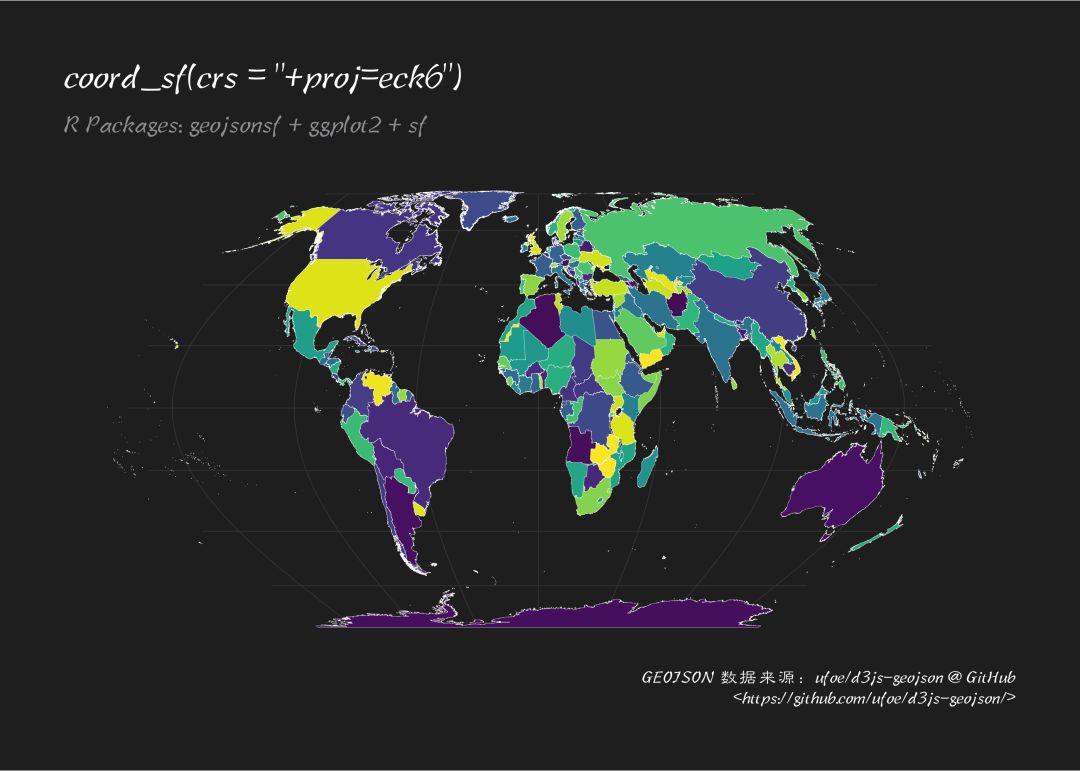
coord_sf(crs = “+proj=eck*”): 我蛮喜欢用这个的
for(i in 1:6){ print(p + coord_sf(crs = paste0("+proj=eck", i)) + labs(title = paste0('coord_sf(crs = "+proj=eck', i, '")')))}