0. 内容
前面四讲都是基础内容,现在开始讲解一些具体的SLAM的内容。
视觉里程计有两种方法:特征点法和直接法,本次讲特征点法。
1. 特征点

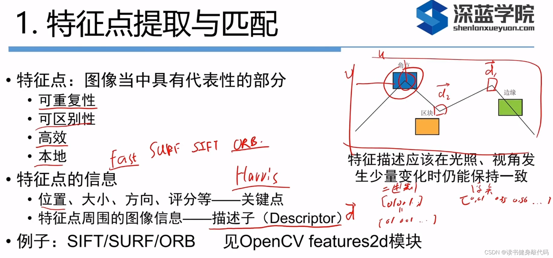
实际中的描述子用二进制的比较多,好计算且内存小。
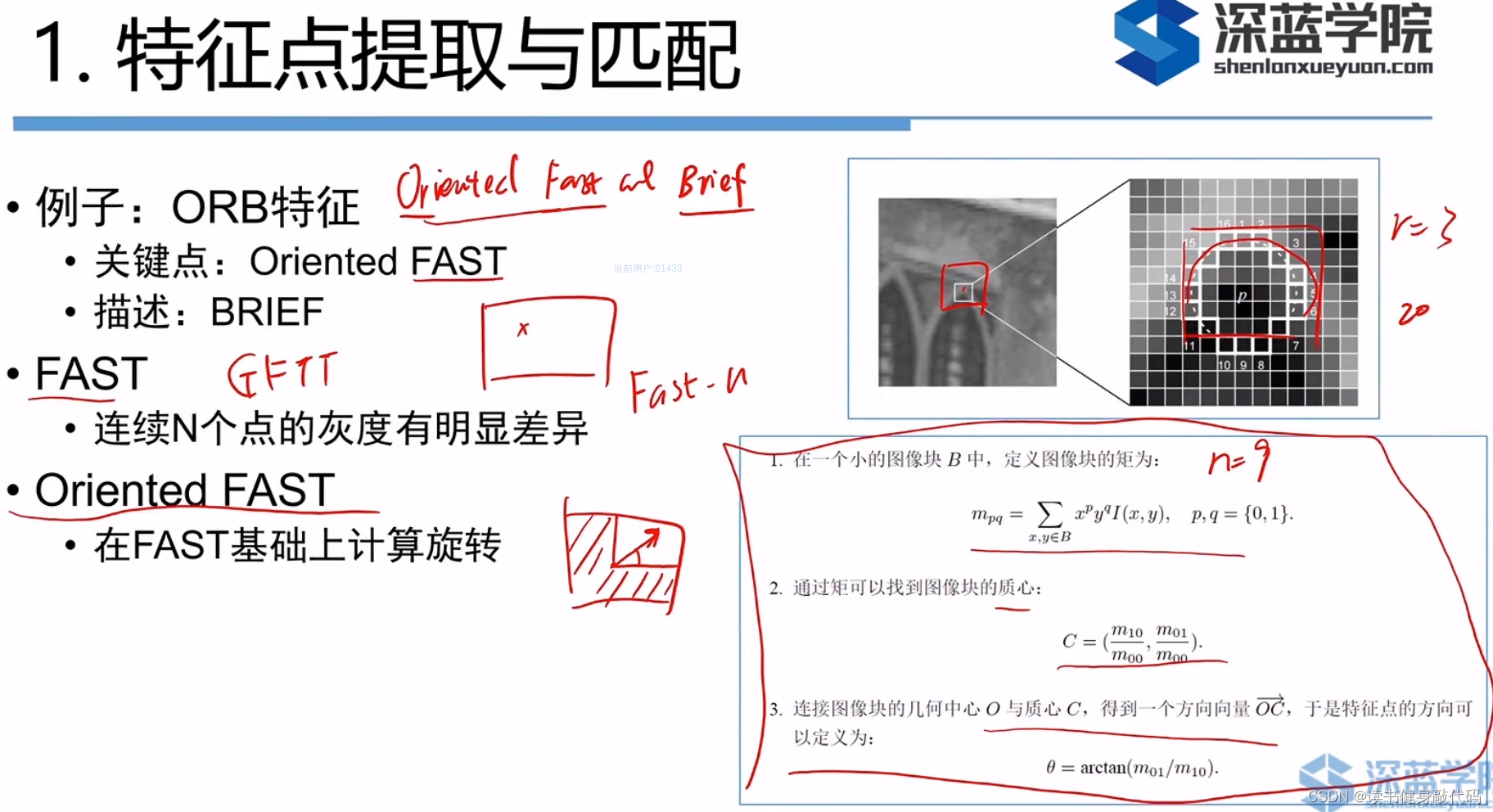
1. FAST关键点
特征点相关:以ORB为例
连续n(如取9个)个点的像素的亮度逗比改点像素的亮度大/小一个阈值(如20),这时认为是关键点,否则认为不是,则这种特征点就叫FAST-9,还有FAST-11用的也较多。
FAST的优势是提取的速度很快,缺点是不是很精确,容易扎堆,一般提取完之后要进行以下非最大值抑制,仅保留响应极大值的角点。
2. BRIEF描述子
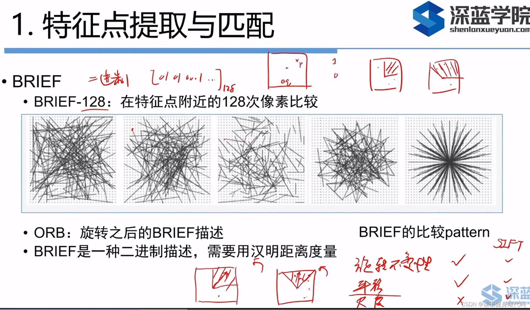
随机选择和按照一定的规则选择结果不会相差很大。
3. 特征匹配

暴力匹配
、只匹配某些区域内的点、一些加速算法,如
快速最近邻
。
2. 2D-2D对极几何
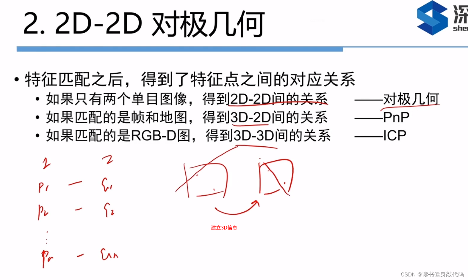
所有的算法当中,2D-2D是最难的,因为知道的信息最少。
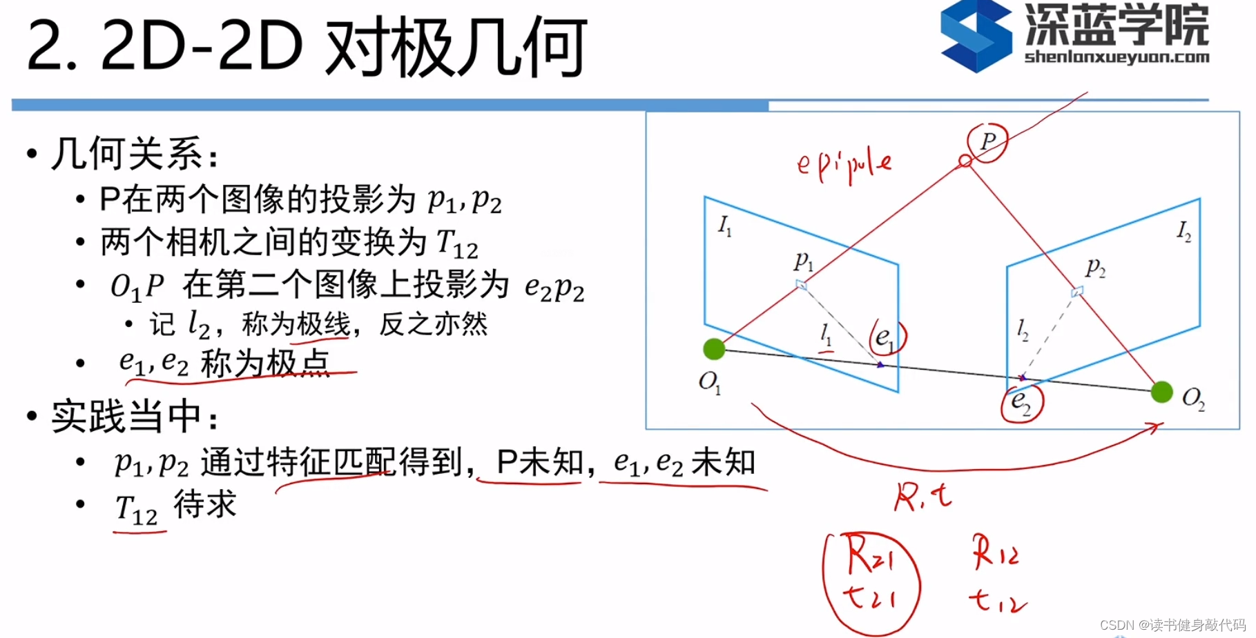
注意用的旋转矩阵的方向,从哪个到哪个。
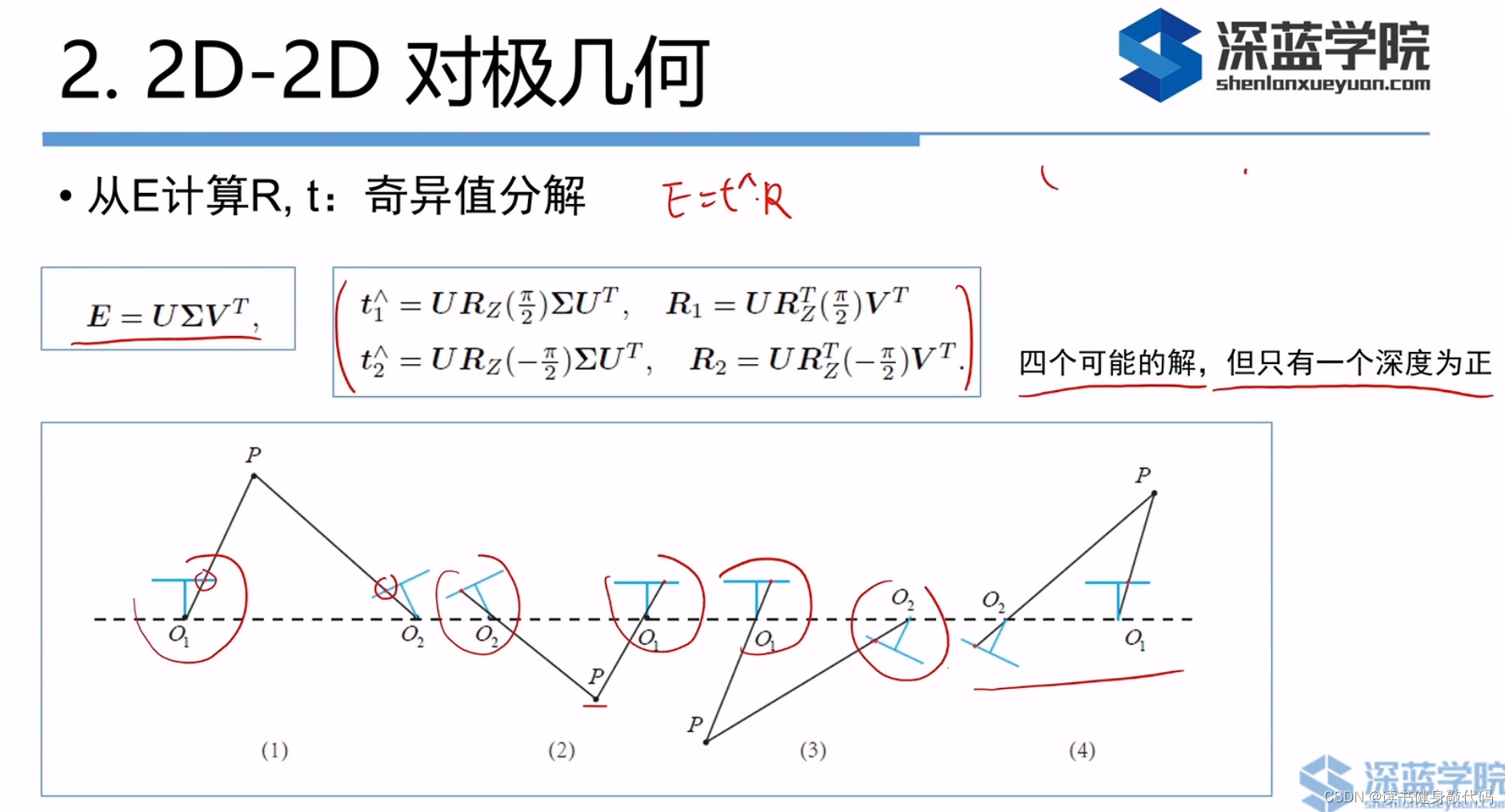
2*2有4个可能的解,但是深度只能为正,所以最后只有一个正确的解。

对八点法进行了一些讨论:
目的是对单目进行init,
确定尺度,纯旋转无法init问题,
尺度不确定性问题(t只代表方向,尺度t变大或者缩小时,观测点的相对位置不变),还可能出现尺度漂移,
以及估计的R,t不对时,使用RANSAC检测,重新估计(RANSAC思路:200对匹配点中取8对计算R,t,用剩下的192对去验证,如果大部分,如160对都符合,则R,t可能对,如果只有很少的符合(可能8对点中有误匹配的外点),如20对,则可能错,重新选8对,再计算R,t,总会找到合适的8对点)
还有一种情况:
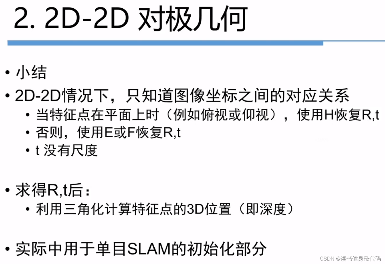
当场景中的特征点都落在同一个平面上,那么两张图中的位置之间存在直接的线性关系,这个关系可以用矩阵来描述,这个矩阵就是单应矩阵(Homography),常用于无人机这种相机看到的场景提取出来的特征点都在同一平面。

通过匹配出来的点算出H(据说是4组点)->R,t
实际中E和H这两种方式都会尝试一下,看哪种好用就用哪种。
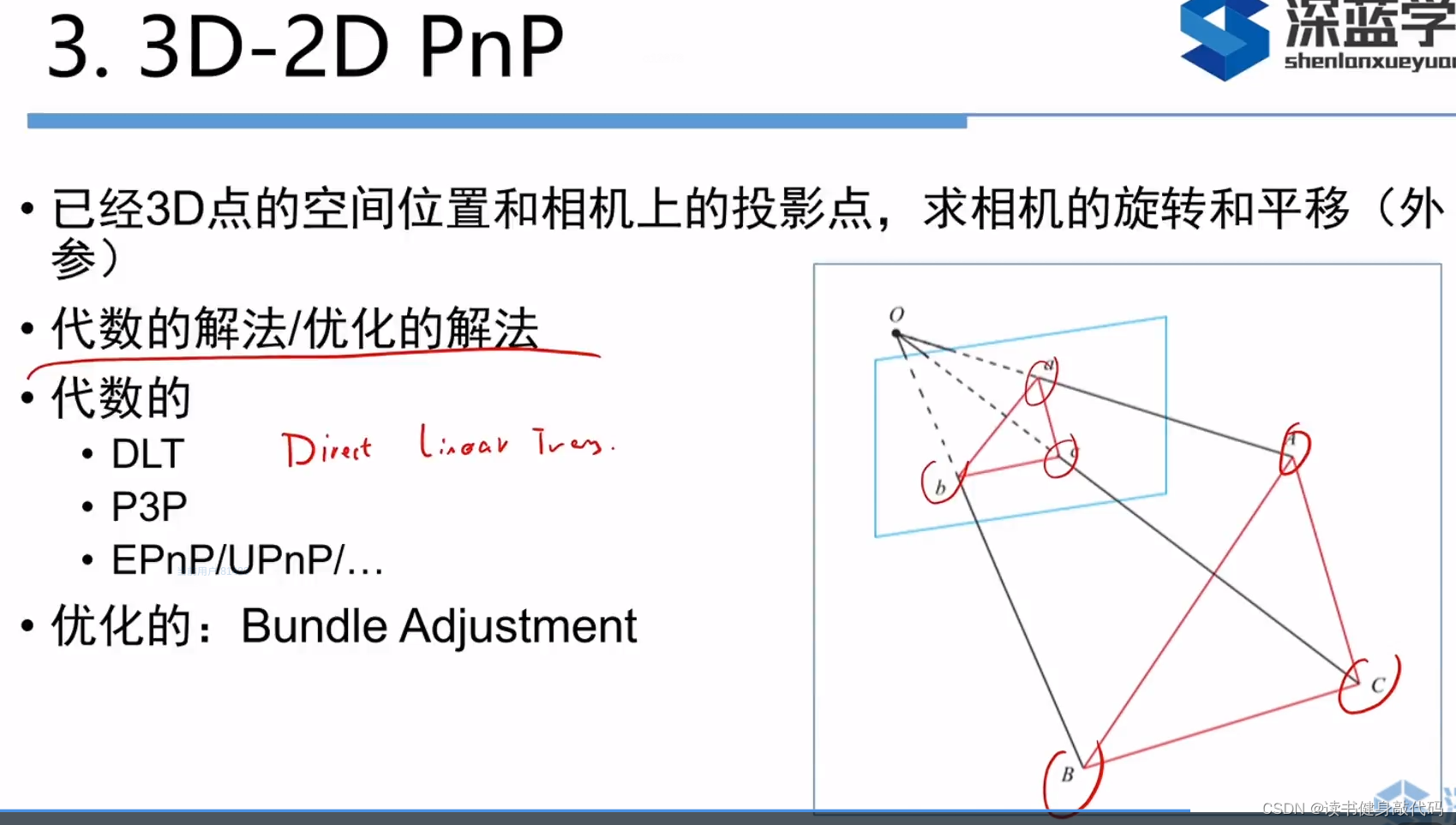
3. 3D-2D PnP
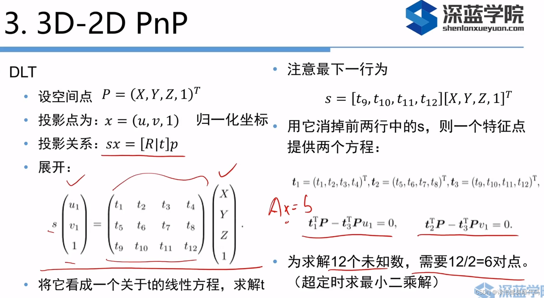
1. DLT(直接线性变换法)
当已知空间当中的投影点和空间中的深度信息时,用PnP方法求相机外参。
这里和算E,F,H矩阵挺像的,
方程组12个未知数,一对点提供两个方程,需要12/2=6对点。
转化为求解线性方程组。
3. P3P法
书上写了。
EPnP,UPnP有兴趣看,没兴趣会调用,知道是啥即可。
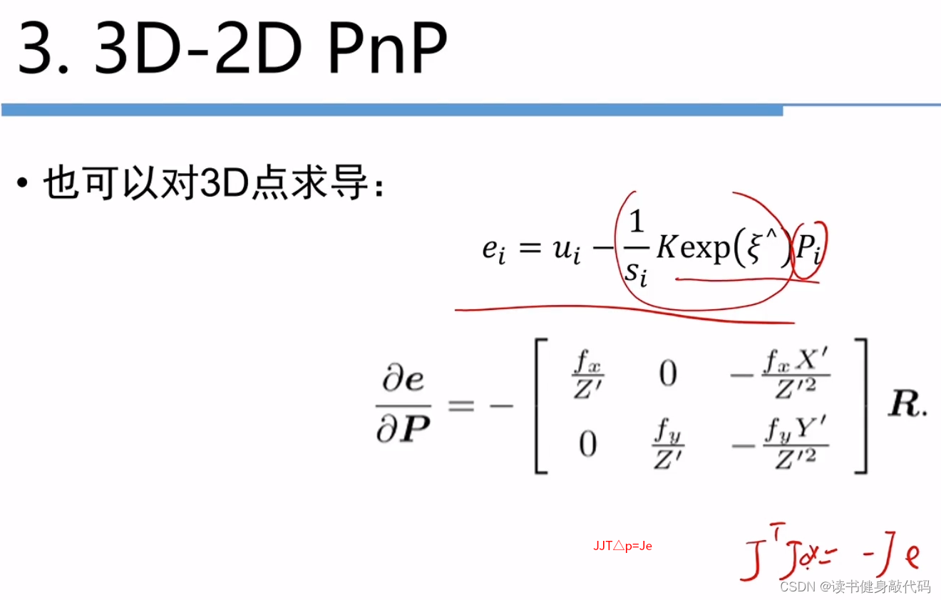
2. 使用最小化重投影误差的方法来求解PnP(BA方法)
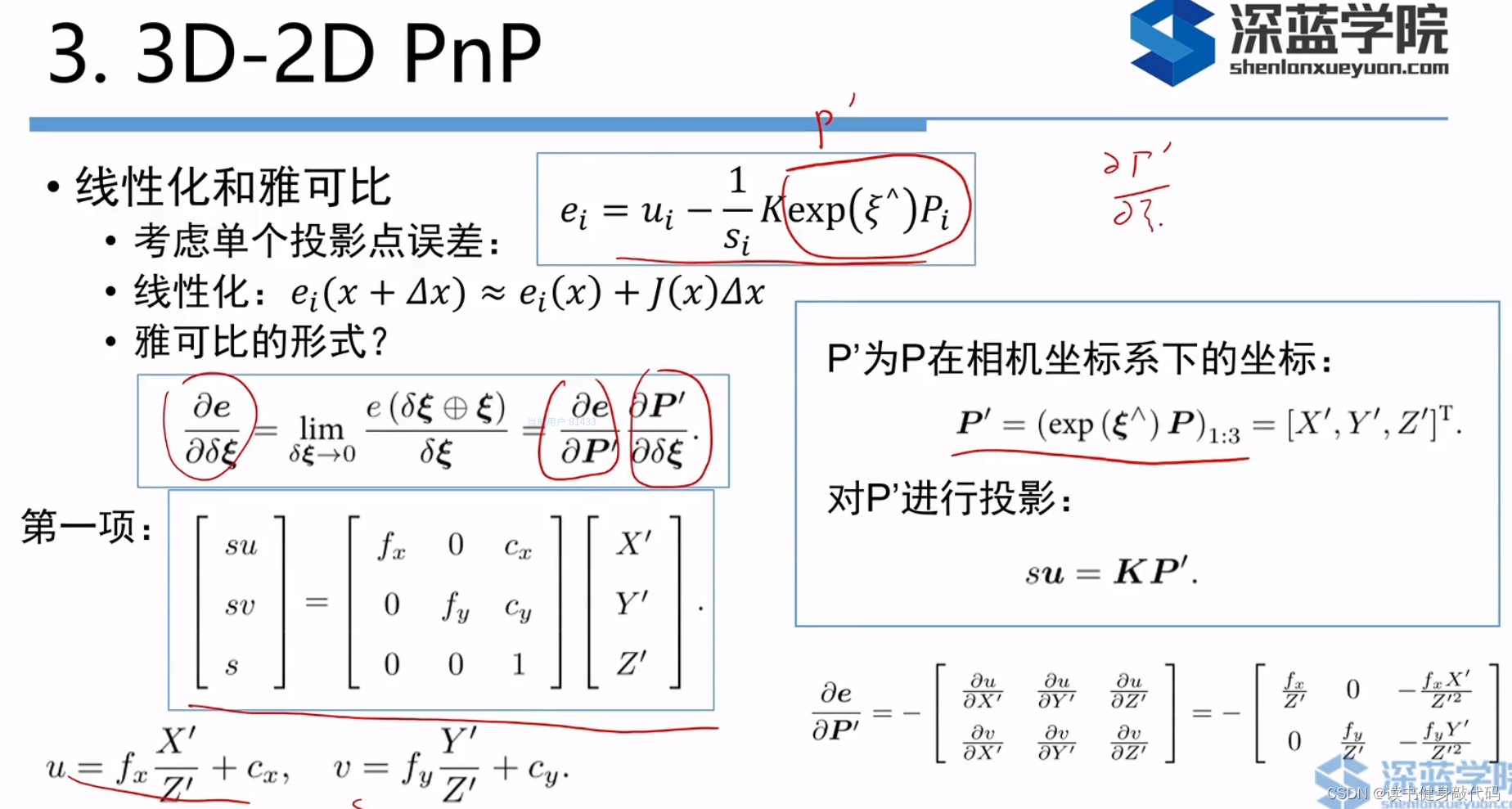
这部分数学很多。
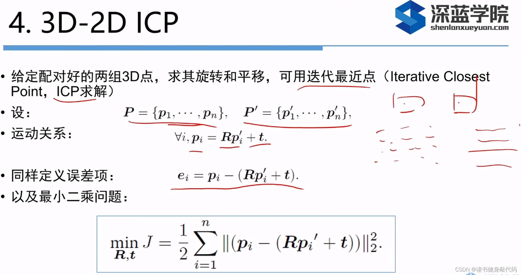
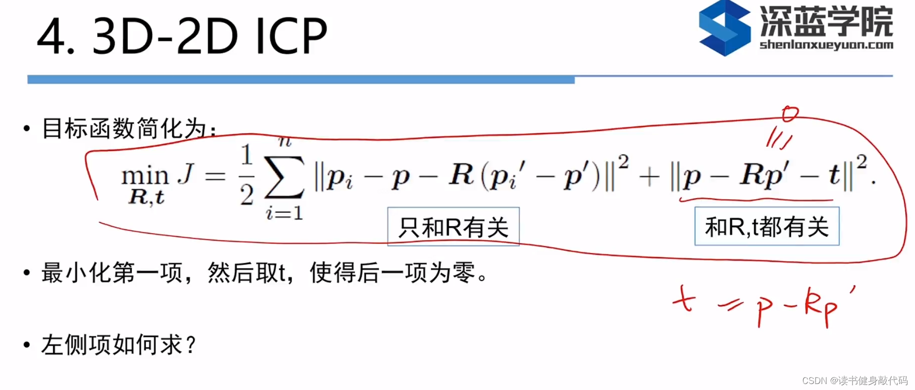
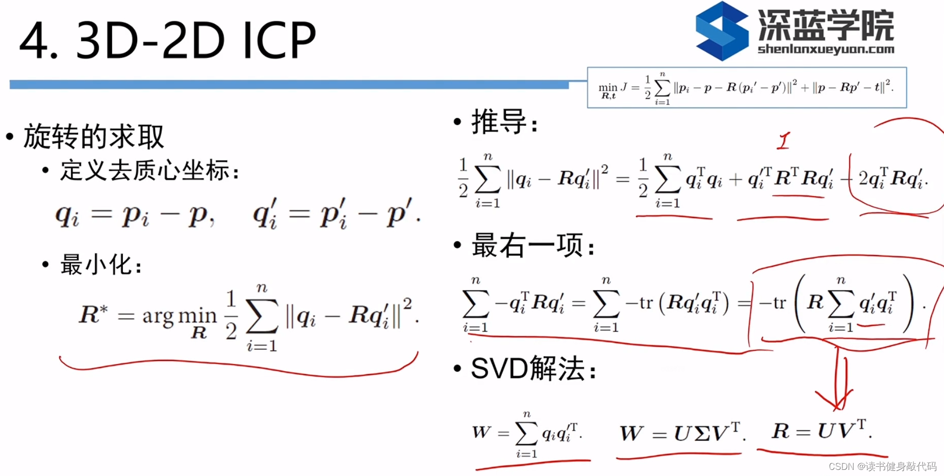
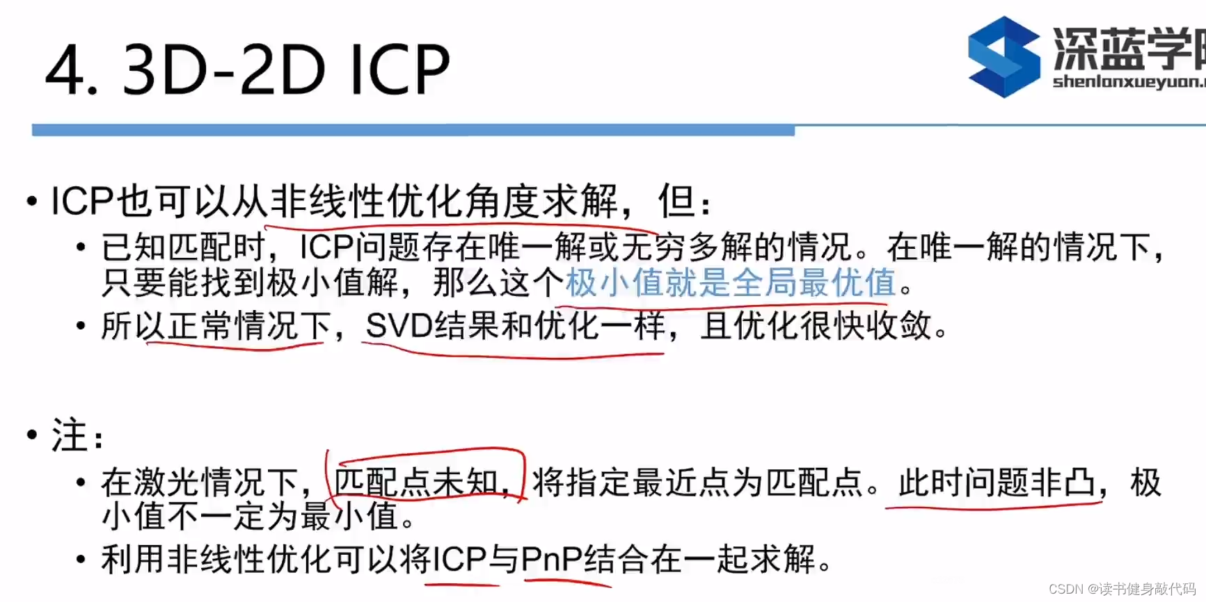
4. 3D-3D ICP
5. 三角测量(单目深度恢复)
对不同位置观测到的路标点进行特征匹配,使用几何关系求得路标点在两个左右相机坐标系下的深度值,就是三角测量。
教材上的代码为:使用了OpenCV的
cv::triangulatePoints
函数,传入匹配成功的特征点,通过三角测量计算出这些特征点在
I
1
I_1
I
1
相机系下的深度值(按理来说应该可以同时得到
I
1
I_1
I
1
和
I
2
I_2
I
2
的深度值,无需借助估计的变换矩阵,这里应该只是为了验证三角化点与特征点的重投影关系)
void triangulation(
const vector<KeyPoint> &keypoint_1,
const vector<KeyPoint> &keypoint_2,
const std::vector<DMatch> &matches,
const Mat &R, const Mat &t,
vector<Point3d> &points) {
Mat T1 = (Mat_<float>(3, 4) <<
1, 0, 0, 0,
0, 1, 0, 0,
0, 0, 1, 0);
Mat T2 = (Mat_<float>(3, 4) <<
R.at<double>(0, 0), R.at<double>(0, 1), R.at<double>(0, 2), t.at<double>(0, 0),
R.at<double>(1, 0), R.at<double>(1, 1), R.at<double>(1, 2), t.at<double>(1, 0),
R.at<double>(2, 0), R.at<double>(2, 1), R.at<double>(2, 2), t.at<double>(2, 0)
);
Mat K = (Mat_<double>(3, 3) << 520.9, 0, 325.1, 0, 521.0, 249.7, 0, 0, 1);
vector<Point2f> pts_1, pts_2;
for (DMatch m:matches) {
// 将像素坐标转换至相机坐标
pts_1.push_back(pixel2cam(keypoint_1[m.queryIdx].pt, K));
pts_2.push_back(pixel2cam(keypoint_2[m.trainIdx].pt, K));
}
Mat pts_4d;
cv::triangulatePoints(T1, T2, pts_1, pts_2, pts_4d); //返回的是特征点三角测量之后的其次坐标,将其归一化为最后一维为1就可以取前三维为非其次坐标
// 转换成非齐次坐标
for (int i = 0; i < pts_4d.cols; i++)
{
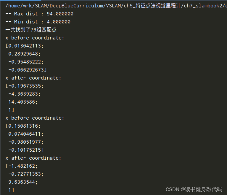
Mat x = pts_4d.col(i);
cout<<"x before coordinate:\n"<<x<<endl;
x /= x.at<float>(3, 0); // 归一化
cout<<"x after coordinate:\n"<<x<<endl;
Point3d p(
x.at<float>(0, 0),
x.at<float>(1, 0),
x.at<float>(2, 0)
);
points.push_back(p);
}
}
三角化之后的结果是4
N的矩阵,每一列都是4
1的齐次坐标,需要归一化取得非其次坐标(最后一维为1,见教材
P
46
P_{46}
P
4
6
)。
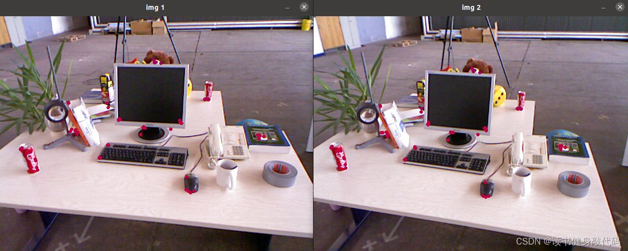
三角化点与特征点的重投影关系,对得到的I1的深度值使用变换T,得到了I2中的深度值
  //-- 验证三角化点与特征点的重投影关系
  Mat K = (Mat_<double>(3, 3) << 520.9, 0, 325.1, 0, 521.0, 249.7, 0, 0, 1);
  Mat img1_plot = img_1.clone();
  Mat img2_plot = img_2.clone();
  for (int i = 0; i < matches.size(); i++)
  {
    // 第一个图
    float depth1 = points[i].z;
    cout << "depth: " << depth1 << endl;
    Point2d pt1_cam = pixel2cam(keypoints_1[matches[i].queryIdx].pt, K);
    cv::circle(img1_plot, keypoints_1[matches[i].queryIdx].pt, 2, get_color(depth1), 2);

    // 第二个图()
    Mat pt2_trans = R * (Mat_<double>(3, 1) << points[i].x, points[i].y, points[i].z) + t;
    float depth2 = pt2_trans.at<double>(2, 0);
    cv::circle(img2_plot, keypoints_2[matches[i].trainIdx].pt, 2, get_color(depth2), 2);
  }
  cv::imshow("img 1", img1_plot);
  cv::imshow("img 2", img2_plot);
  cv::waitKey();
使用重投影验证三角化结果,证明三角化整体是对的。
但是三角测量存在以下问题:
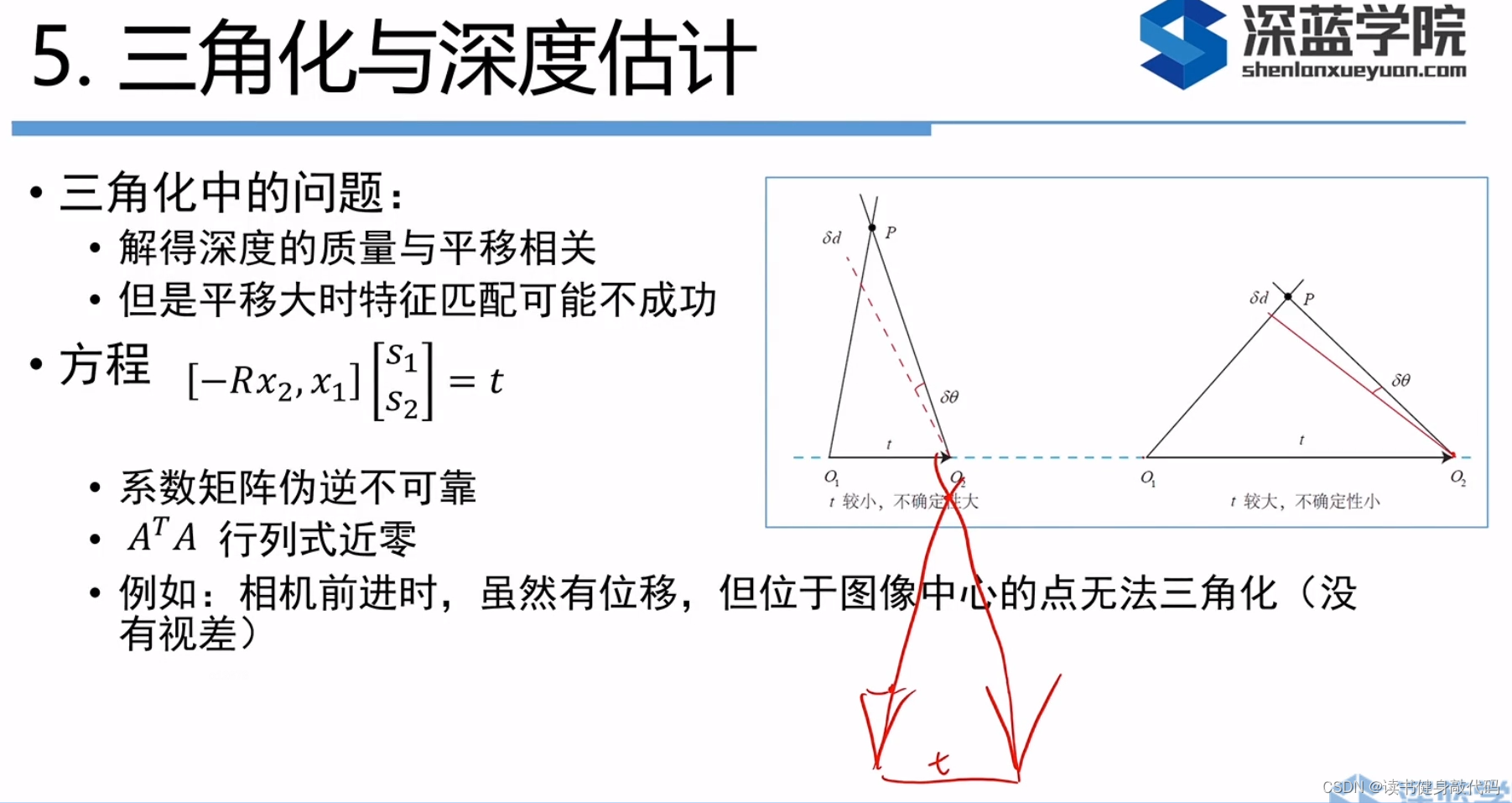
单目需要依靠平移来进行三角测量,当平移量小时,三角化的精度不够;平移量大时,被物体发生的变化可能较大,可能导致匹配失败。这就是三角化的矛盾,被称为“”视差(parallax)。可以计算每个特征点的位置和不确定性,不断观测,方差减小并收敛,即为深度滤波器(在建图部分的单目稠密重建讲到)。
6. 实践环节
feature_extraction
看
opencv文档
1. 2D-2D结果,对极几何
-- Max dist : 94.000000
-- Min dist : 4.000000
一共找到了79组匹配点
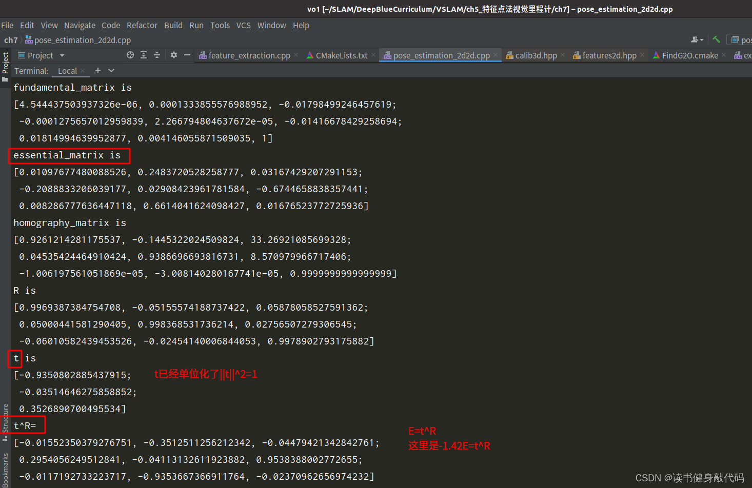
fundamental_matrix is
[4.544437503937326e-06, 0.0001333855576988952, -0.01798499246457619;
-0.0001275657012959839, 2.266794804637672e-05, -0.01416678429258694;
0.01814994639952877, 0.004146055871509035, 1]
essential_matrix is
[0.01097677480088526, 0.2483720528258777, 0.03167429207291153;
-0.2088833206039177, 0.02908423961781584, -0.6744658838357441;
0.008286777636447118, 0.6614041624098427, 0.01676523772725936]
homography_matrix is
[0.9261214281175537, -0.1445322024509824, 33.26921085699328;
0.04535424464910424, 0.9386696693816731, 8.570979966717406;
-1.006197561051869e-05, -3.008140280167741e-05, 0.9999999999999999]
R is
[0.9969387384754708, -0.05155574188737422, 0.05878058527591362;
0.05000441581290405, 0.998368531736214, 0.02756507279306545;
-0.06010582439453526, -0.02454140006844053, 0.9978902793175882]
t is
[-0.9350802885437915;
-0.03514646275858852;
0.3526890700495534]
t^R=
[-0.01552350379276751, -0.3512511256212342, -0.04479421342842761;
0.2954056249512841, -0.04113132611923882, 0.9538388002772655;
-0.0117192733223717, -0.9353667366911764, -0.02370962656974232]
epipolar constraint = [-0.0005415187881110395]
epipolar constraint = [-0.002158321995511289]
epipolar constraint = [0.0003344241044139079]
epipolar constraint = [-8.762782289159499e-06]
epipolar constraint = [0.000212132191399178]
epipolar constraint = [0.0001088766997727197]
epipolar constraint = [0.0004246621771667111]
epipolar constraint = [-0.003173128212208817]
epipolar constraint = [-3.716645801081497e-05]
epipolar constraint = [-0.001451851842241985]
epipolar constraint = [-0.0009607717979376318]
epipolar constraint = [-0.0008051993498427168]
epipolar constraint = [-0.001424813546545535]
epipolar constraint = [-0.0004339424745821371]
epipolar constraint = [-0.000478610965853582]
epipolar constraint = [-0.000196569283305803]
epipolar constraint = [0.001542309777196771]
epipolar constraint = [0.003107154828888181]
epipolar constraint = [0.0006774648890596965]
epipolar constraint = [-0.001176167495933316]
epipolar constraint = [-0.003987986032032258]
epipolar constraint = [-0.001255263863164498]
epipolar constraint = [-0.001553941958847024]
epipolar constraint = [0.002009914869739976]
epipolar constraint = [-0.0006068096307232096]
epipolar constraint = [-2.769881004420494e-05]
epipolar constraint = [0.001274573011402158]
epipolar constraint = [-0.004169986054360234]
epipolar constraint = [-0.001108104733689524]
epipolar constraint = [-0.0005154295520383712]
epipolar constraint = [-0.001776993208794389]
epipolar constraint = [6.677362292956124e-07]
epipolar constraint = [-0.001853977732928294]
epipolar constraint = [-0.0004823070333038748]
epipolar constraint = [0.0004740904480800279]
epipolar constraint = [-0.002961041748859255]
epipolar constraint = [-0.003347655248297339]
epipolar constraint = [-0.0001975680967504778]
epipolar constraint = [-0.002824643387150695]
epipolar constraint = [-0.0004311798170555103]
epipolar constraint = [0.001181203684013504]
epipolar constraint = [1.756266610475343e-07]
epipolar constraint = [-0.002137829859245668]
epipolar constraint = [0.001153415527396465]
epipolar constraint = [-0.002120357728713398]
epipolar constraint = [2.741529055910741e-06]
epipolar constraint = [0.000904458201820401]
epipolar constraint = [-0.002100484435898768]
epipolar constraint = [-0.0003517789219357401]
epipolar constraint = [-2.72046484559238e-05]
epipolar constraint = [-0.003784823353263345]
epipolar constraint = [-0.001588562608841583]
epipolar constraint = [-0.002928516011805465]
epipolar constraint = [-0.001016592266471106]
epipolar constraint = [0.0001241874577868896]
epipolar constraint = [-0.0009797104629406181]
epipolar constraint = [0.001457875224685545]
epipolar constraint = [-1.153738078288336e-05]
epipolar constraint = [-0.00273324742758773]
epipolar constraint = [0.00141572125781092]
epipolar constraint = [0.001790255871328722]
epipolar constraint = [-0.002547929671675515]
epipolar constraint = [-0.006257078861794559]
epipolar constraint = [-0.001874877415315751]
epipolar constraint = [-0.002104542912833518]
epipolar constraint = [1.39253152928176e-06]
epipolar constraint = [-0.004013502582090489]
epipolar constraint = [-0.004726241071896793]
epipolar constraint = [-0.001328682673648302]
epipolar constraint = [3.995925173527759e-07]
epipolar constraint = [-0.005080511723986339]
epipolar constraint = [-0.001977141850700581]
epipolar constraint = [-0.00166133426468739]
epipolar constraint = [0.004285762870626424]
epipolar constraint = [0.004087325194305855]
epipolar constraint = [0.0001482534285787533]
epipolar constraint = [-0.000962530113462208]
epipolar constraint = [-0.002341076011427135]
epipolar constraint = [-0.006138005035457875]
2. 3D-2D结果,调用PnP函数
这里的t是精确的,是带尺度的。
wrk@MyPC:~/SLAM/DeepBlueCurriculum/VSLAM/ch5_特征点法视觉里程计/ch7_slambook2/cmake-build-debug$ ./pose_estimation_3d2d 1.png 2.png 1_depth.png 2_depth.png
-- Max dist : 94.000000
-- Min dist : 4.000000
一共找到了79组匹配点
3d-2d pairs: 75
solve pnp in opencv cost time: 0.000188566 seconds.
R=
[0.9978745555297591, -0.05102729297915373, 0.04052883908410459;
 0.04983267620066928, 0.9983081506312504, 0.02995898472731967;
 -0.04198899628432293, -0.02787564805402974, 0.9987291286613218]
t=
[-0.1273034869580363;
 -0.01157187487421139;
 0.05667408337434332]
calling bundle adjustment by gauss newton
iteration 0 cost=40517.7576706
iteration 1 cost=410.547029116
iteration 2 cost=299.76468142
iteration 3 cost=299.763574327
pose by g-n:
   0.997905909549  -0.0509194008562   0.0398874705187   -0.126782139096
   0.049818662505    0.998362315745   0.0281209417649 -0.00843949683874
 -0.0412540489424  -0.0260749135374    0.998808391199   0.0603493575229
                0                 0                 0                 1
solve pnp by gauss newton cost time: 7.4831e-05 seconds.
calling bundle adjustment by g2o
iteration= 0     chi2= 410.547029        time= 1.7213e-05        cumTime= 1.7213e-05     edges= 75       schur= 0
iteration= 1     chi2= 299.764681        time= 1.2173e-05        cumTime= 2.9386e-05     edges= 75       schur= 0
iteration= 2     chi2= 299.763574        time= 9.498e-06         cumTime= 3.8884e-05     edges= 75       schur= 0
iteration= 3     chi2= 299.763574        time= 8.225e-06         cumTime= 4.7109e-05     edges= 75       schur= 0
iteration= 4     chi2= 299.763574        time= 9.427e-06         cumTime= 5.6536e-05     edges= 75       schur= 0
iteration= 5     chi2= 299.763574        time= 8.055e-06         cumTime= 6.4591e-05     edges= 75       schur= 0
iteration= 6     chi2= 299.763574        time= 7.925e-06         cumTime= 7.2516e-05     edges= 75       schur= 0
iteration= 7     chi2= 299.763574        time= 8.016e-06         cumTime= 8.0532e-05     edges= 75       schur= 0
iteration= 8     chi2= 299.763574        time= 8.175e-06         cumTime= 8.8707e-05     edges= 75       schur= 0
iteration= 9     chi2= 299.763574        time= 8.737e-06         cumTime= 9.7444e-05     edges= 75       schur= 0
optimization costs time: 0.000296681 seconds.
pose estimated by g2o =
    0.99790590955  -0.0509194008911   0.0398874704367   -0.126782138956
  0.0498186625425    0.998362315744   0.0281209417542 -0.00843949681823
 -0.0412540488609  -0.0260749135293    0.998808391203   0.0603493574888
                0                 0                 0                 1
solve pnp by g2o cost time: 0.00041274 seconds.
3. 3D-3D,ICP算法
分别使用SVD方法和BA的方法(非线性优化)实现了一遍,本身这个问题是有解析解的,所以BA的方法不是必要的,但是可以看出结果是一样的,且优化了两轮就收敛了。
-- Max dist : 94.000000
-- Min dist : 4.000000
一共找到了79组匹配点
3d-3d pairs: 72
W=  10.871 -1.01948  2.54771
-2.16033  3.85307 -5.77742
 3.94738 -5.79979  9.62203
U=  0.558087  -0.829399 -0.0252034
 -0.428009  -0.313755   0.847565
  0.710878   0.462228   0.530093
V=  0.617887  -0.784771 -0.0484806
 -0.399894  -0.366747   0.839989
  0.676979   0.499631   0.540434
ICP via SVD results:
R = [0.9969452349468715, 0.05983347698056557, -0.05020113095482046;
 -0.05932607657705309, 0.9981719679735133, 0.01153858699565957;
 0.05079975545906246, -0.008525103184062521, 0.9986724725659557]
t = [0.144159841091821;
 -0.06667849443812729;
 -0.03009747273569774]
R_inv = [0.9969452349468715, -0.05932607657705309, 0.05079975545906246;
 0.05983347698056557, 0.9981719679735133, -0.008525103184062521;
 -0.05020113095482046, 0.01153858699565957, 0.9986724725659557]
t_inv = [-0.1461462958593589;
 0.05767443542067568;
 0.03806388018483625]
calling bundle adjustment
iteration= 0     chi2= 1.816112  time= 3.2451e-05        cumTime= 3.2451e-05     edges= 72       schur= 0        lambda= 0.000758        levenbergIter= 1
iteration= 1     chi2= 1.815514  time= 2.684e-05         cumTime= 5.9291e-05     edges= 72       schur= 0        lambda= 0.000505        levenbergIter= 1
iteration= 2     chi2= 1.815514  time= 1.8555e-05        cumTime= 7.7846e-05     edges= 72       schur= 0        lambda= 0.000337        levenbergIter= 1
iteration= 3     chi2= 1.815514  time= 1.8244e-05        cumTime= 9.609e-05      edges= 72       schur= 0        lambda= 0.000225        levenbergIter= 1
iteration= 4     chi2= 1.815514  time= 1.7342e-05        cumTime= 0.000113432    edges= 72       schur= 0        lambda= 0.000150        levenbergIter= 1
iteration= 5     chi2= 1.815514  time= 1.5409e-05        cumTime= 0.000128841    edges= 72       schur= 0        lambda= 0.000100        levenbergIter= 1
iteration= 6     chi2= 1.815514  time= 1.5179e-05        cumTime= 0.00014402     edges= 72       schur= 0        lambda= 0.000067        levenbergIter= 1
iteration= 7     chi2= 1.815514  time= 2.5178e-05        cumTime= 0.000169198    edges= 72       schur= 0        lambda= 0.068117        levenbergIter= 4
optimization costs time: 0.000460198 seconds.

after optimization:
T=
  0.996945  0.0598335 -0.0502011    0.14416
-0.0593261   0.998172  0.0115386 -0.0666785
 0.0507998 -0.0085251   0.998672 -0.0300979
         0          0          0          1
p1 = [-0.0374123, -0.830816, 2.7448]
p2 = [-0.0111479, -0.746763, 2.7652]
(R*p2+t) = [-0.05045153727143986;
 -0.7795087351232993;
 2.737231009770682]

p1 = [-0.243698, -0.117719, 1.5848]
p2 = [-0.297211, -0.0956614, 1.6558]
(R*p2+t) = [-0.24099014946244;
 -0.125427050612953;
 1.609221205035477]

p1 = [-0.627753, 0.160186, 1.3396]
p2 = [-0.709645, 0.159033, 1.4212]
(R*p2+t) = [-0.6251478077232009;
 0.1505624178119533;
 1.351809862712792]

p1 = [-0.323443, 0.104873, 1.4266]
p2 = [-0.399079, 0.12047, 1.4838]
(R*p2+t) = [-0.3209806217783838;
 0.09436777718271656;
 1.430432194554881]

p1 = [-0.627221, 0.101454, 1.3116]
p2 = [-0.709709, 0.100216, 1.3998]
(R*p2+t) = [-0.6276559234155776;
 0.09161021993899245;
 1.330936372911853]
4. 三角测量
在使用对极几何得到相机的运动之后,还需要估计地图点的深度,需要用到三角测量(三角化)

7. 小结