How to Estimate Efficiency?
效率可以通过多种方式衡量; 即:
1.更少的内存利用率
2.更快的执行时间
3.更快释放分配的资源等等
那么如何衡量效率?
测量应独立于所使用的软件(即编译器,语言等)和硬件(CPU速度,内存大小等), 特别是,运行时分析可能存在严重的缺陷,但效率在很大程度上取决于方法的定义。
因此,最好是可以通过直接研究方法定义来执行的抽象分析。
忽略各种限制; 即:CPU速度,内存限制等。
由于该方法现在与特定的计算机环境无关,因此我们将其称为算法。
Estimating Running Time
如何根据算法的定义来估计运行/执行时间?将算法跟踪中执行的语句数视为运行时需求的度量。这个度量可以表示为问题“大小”的函数。算法的运行时间通常随输入的大小而增长。
我们关注运行时间的最坏情况,因为这对许多应用程序至关重要。
给定一个大小为n的问题的方法,找到WordStestn(n),考虑所有可能的参数/输入值。
Example:
Assume an array a [0 … n –1] of int, and assume the following trace:
for (int i = 0; i < n – 1; i++)
if (a [i] > a [i + 1])
System.out.println (i);
What is worstTime(n)?


a = Time taken by the fastest primitive operation
b = Time taken by the slowest primitive operation
Let T(n) be the running time of compareValues. Then
a (4n – 4) <= T(n) <= b(4n – 4)
因此,运行时间T(n)由两个线性函数限定

Constant Factors
增长率不受以下因素影响
1. 常数
2. 低阶项
Examples
-
102? + 105 is a linear function

-
105?2 + 108? is a quadratic function

使用极限的思想来理解这段话
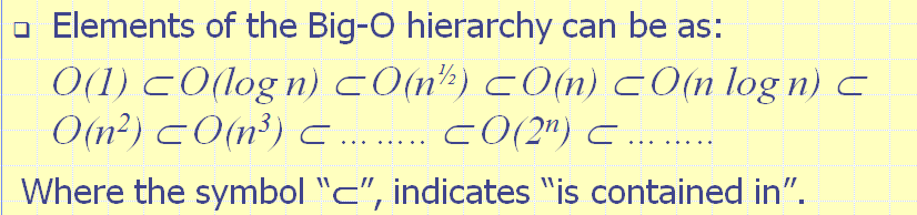
Big-O Notation
我们不需要计算确切的最坏时间,因为它只是时间要求的近似值。相反,我们可以用“Big-O”表示法来近似那个时间。这是相当令人满意的,因为它给了我们近似的近似值!基本思想是确定算法/功能行为的上限。换句话说,要确定算法的性能有多差!如果某个函数g(n)是函数f(n)的上限,那么我们说f(n)是g(n)的Big-O。
(原文:The basic idea is to determine an upper bound for the behavior of the algorithm/function. In other words, to determine how bad the performance of the algorithm can get!If some function g(n) is an upper bound of function f(n), then we say that f(n) is Big-O of g(n). )
基本思想是确定算法/功能行为的上限。换句话说,要确定算法的性能有多差!
如果某个函数g(n)是函数f(n)的上限,那么我们说f(n)是g(n)的Big-O。
具体来说,Big-O的定义如下:给定函数f(n)和g(n),如果存在正常数c和n0,则f(n)为O(g(n)),这样
对于n> = n0,f(n)<= c*g(n)


但是,尽管事实上f2(n)的顺序比f1(n)的顺序高/最差,但对于所有小于10,000的n值,f1(n)实际上大于f2(n)!


Asymptotic Algorithm Analysis
In computer science and applied mathematics, asymptotic analysis is a way of describing limiting behaviours (may approach ever nearer but never crossing!).
Asymptotic analysis of an algorithm determines the running time in big-O notation. To perform the asymptotic analysis:
– We find the worst-case number of primitive operations executed as a function of the input size
– We then express this function with big-O notation
在计算机科学和应用数学中,渐近分析是描述限制行为的一种方法(可能会越来越近,但永不过分!)。
算法的渐近分析确定了big-O表示法的运行时间。 要执行渐近分析:
-我们发现最坏情况下执行的原始操作数是输入大小的函数
-然后,我们使用big-O表示法表达此功能
Example:
We determine that algorithm compareValues executes at most 4n – 4 primitive operations
We say that algorithm compareValues “runs in O(n) time”, or has a “complexity” of O(n)
Note: Since constant factors and lower-order terms are eventually dropped anyhow, we can disregard them when counting primitive operations
If two algorithms A & B exist for solving the same problem, and, for instance, A is O(n) and B is O(n2), then we say that A is asymptotically better than B (although for a small time B may have lower running time than A).
我们确定算法compareValues最多执行4n-4个原始运算
我们说算法compareValues“运行时间为O(n)”,或者具有“复杂度”为O(n)
注意:由于常量因数和低阶项最终都会被丢弃,因此在计算原始运算时可以忽略它们
如果存在用于解决同一问题的两种算法A和B,例如A为O(n)而B为O(n2),则我们说A渐近优于B(尽管在很短的时间内B可能 具有比A更低的运行时间。
To illustrate the importance of the asymptotic point of view, let us consider three algorithms that perform the same operation, where the running time (in µs) is as follows, where n is the size of the problem:
Algorithm1: 400n
Algorithm2: 2n^2
Algorithm3: 2^n
Which of the three algorithms is faster?
Notice that Algorithm1 has a very large constant factor compared to the other two algorithms!
为了说明渐近观点的重要性,让我们考虑执行相同操作的三种算法,其中运行时间(以μs为单位)如下,其中n是问题的大小:
算法1:400n
算法2:2n ^ 2
算法3:2 ^ n
三种算法中哪种更快?
请注意,与其他两种算法相比,Algorithm1具有非常大的常数因子!
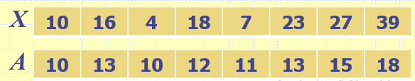
Let us further illustrate asymptotic analysis with two algorithms that would compute prefix averages.
Given an array X storing n numbers, we need to construct an array A such that:
A[i] is the average of X[0] + X[1] + … + X[i])
That is, the i-th prefix average of an array X is average of the first (i + 1) elements of X:
A[i] = (X[0] + X[1] + … + X[i])/(i+1)
Computing prefix average has applications to financial analysis; for instance the average annual return of a mutual fund for the last year, three years, ten years, etc.
让我们进一步说明使用两种算法计算渐进平均值的渐进分析。
给定一个存储n个数字的数组X,我们需要构造一个数组A,使得:
A [i]是X [0] + X [1] +…+ X [i]的平均值)
也就是说,数组X的第i个前缀平均值是X的第一个(i + 1)元素的平均值:
A [i] =(X [0] + X [1] +…+ X [i])/(i + 1)
计算前缀平均值可应用于财务分析; 例如,共同基金最近一年,三年,十年等的平均年回报率。

Prefix Averages (Quadratic)
The following algorithm computes prefix averages in quadratic time (n^2) by applying the definition
以下算法通过应用定义来计算二次时间(n^2)中的前缀平均值

Hence, to calculate the sum n integers, the algorithm needs (from the segment that has the two loops) n(n + 1) / 2 operations.
In other words, prefixAverages1 is
O(1 + 2 + …+ n) = O(n(n + 1) / 2) è O(n2)
因此,要计算n个整数的总和,该算法需要(从具有两个循环的段中)进行n(n +1)/ 2个运算。
换句话说,prefixAverages1是O(1 + 2 +…+ n)= O(n(n + 1)/ 2)–> O(n^2)
Prefix Averages (Linear)
The following algorithm computes prefix averages in linear time (n) by keeping a running sum
以下算法通过保持运行总和来计算线性时间(n)中的前缀平均值

Algorithm prefixAverages2 runs in O(n) time, which is clearly better than prefixAverages1.
算法prefixAverages2的运行时间为O(n),这明显优于prefixAverages1。
Big-Omega, Big-Theta &
Plain English!
In addition to Big-O, there are two other notations that are used for algorithm analysis: Big-Omega and Big-Theta.
While Big-O provides an upper bound of a function, Big-Omega provides a lower bound.
In other words, while Big-O indicates that an algorithm behavior “cannot be any worse than”, Big-Omega indicates that it “cannot be any better than”.
Logically, we are often interested in worst-case estimations, however knowing the lower bound can be significant when trying to achieve an optimal solution.
除Big-O外,还有其他两种用于算法分析的符号:Big-Omega和Big-Theta。
Big-O提供功能的上限,而Big-Omega提供功能的下限。
换句话说,Big-O表示算法行为“不比”差,Big-Omega表示算法“不比”差。
从逻辑上讲,我们通常对最坏情况的估计很感兴趣,但是知道下限在尝试获得最佳解决方案时可能很重要。
big-Omega
Big-Omega is defined as follows: Given functions f(n) and g(n), we say that f(n) is Ω(g(n)) if there are positive constants c and n0 such that
f(n) >= cg(n) for n >= n0
Big-O provides and upper bound of a function, while Big-Ω provides a lower bound of it.
In many, if not most, cases, there is often a need of one function that would serve as both lower and upper bounds; that is Big-Theta (Big-Θ).
Big-Omega的定义如下:给定函数f(n)和g(n),如果存在正常数c和n0,则说f(n)为Ω(g(n))。
对于n> = n0,f(n)> = cg(n)
Big-O提供函数的上限,而Big-Ω提供函数的下限。
在很多(如果不是大多数)情况下,通常需要一个功能同时充当上下限。 那就是Big-Theta(Big-Θ)。
big-Theta
Big-Theta is defined as follows: Given functions f(n) and g(n), we say that f(n) is Θ(g(n)) if there are positive constants c1, c2 and n0 such that
c1g(n) <= f(n) <= c2g(n) for n >= n0
Simply put, if a function is f(n) is Ω(g(n)), then it is bounded above and below by some constants time g(n); in other words, it is, roughly, bounded above and below by g(n).
Notice that if f(n) is Θ(g(n)), then it is hence both O(g(n)) and Ω(g(n)).
Big-Theta的定义如下:给定函数f(n)和g(n),我们说如果存在正常数c1,c2和n0,则f(n)为Θ(g(n))。
c1g(n)<= f(n)<= c2g(n)对于n> = n0
简而言之,如果一个函数为f(n)为Ω(g(n)),则该函数上下限为某个常数时间g(n); 换句话说,它大致由g(n)上下限制。
注意,如果f(n)是Θ(g(n)),则它既是O(g(n))又是Ω(g(n))。


Plain English
Sometimes, it might be easier to just indicate the behavior of a method through natural language equivalence of Big-Θ.
For instance
if f(n) is Θ(n), we indicate that f is “linear in n”.
if f(n) is Θ(n2), we indicate that f is “quadratic in n”.
The following table shows the English-language equivalence of Big-Θ
有时,通过Big-Θ的自然语言等效性仅指示方法的行为可能会更容易。
例如
如果f(n)是Θ(n),则表明f是“ n线性”。
如果f(n)为Θ(n2),则表明f为“二次方n”。
下表显示了Big-Θ的英语对等

Big-O
We may just prefer to use plain English, such as “linear”, “quadratic”, etc..
However, in practice, there are MANY occasions when all we specify is an upper bound to the method, which is namely:
Big-O

屏幕剪辑的捕获时间: 2020/1/15 9:25
Big-O and Growth Rate
The big-O notation gives an upper bound on the growth rate of a function
The statement “f(n) is O(g(n))” means that the growth rate of f(n) is no more than the growth rate of g(n)
We can use the big-O notation to rank functions according to their growth rate

Again, we are specifically interested in how rapidly a function increases based on its classification.
For instance, suppose that we have a method whose worstTime() estimate is linear in n, what will be the effect of doubling the problem size?
worstTime(n) ≈ c * n, for some constant c, and sufficiently large value of n
If the problem size doubles then worstTime(n) ≈ c * 2n ≈ 2* worstTime(n)
In other words, if n is doubled, then worst time is doubled.
Now, suppose that we have a method whose worstTime() estimate is quadratic in n, what will be the effect of doubling the problem size?
worstTime(n) ≈ c * n2
If the problem size doubles then worstTime(2n) ≈ c * (2n)2 = c * 4 * n2 ≈ 4* worstTime(n)
In other words, if n is doubled, then worst time is quadrupled.

Again, remember that the Big-O differences eventually dominate constant factors.
For instance if n is sufficiently large, 100 n log n will still be smaller than n2 / 100.
So, the relevance of Big-O, Big-W or Bog-Q may actually depend on how large the problem size may get (i.e. 100,000 or more in the above example).
The following table provides estimate of needed execution time for various functions of n, if n = 1000,000,000, running on a machine executing 1000,1000 statements per second.

