博客

Lecture 3:Real-Time Shadows 1

• Recap: shadow mapping
  
  [slides courtesy of Prof. Ravi Ramamoorthi]

  Issues from shadow mapping and solutions

• The math behind shadow mapping

• Percentage closer soft shadows

一、Shadow Mapping

• A 2-Pass Algorithm

  –The light pass generates the SM

  –The camera pass uses the SM (recall last lecture)

  shadow mapping是一个两趟的算法（渲染场景两遍），第一遍从光源看向场景，输出距离光源最近的最浅深度shadow map，第二遍从相机位置看向场景，配合刚刚的生成的最浅深度图shadow map，渲染出结果。

• An image-space algorithm

  –Pro: no knowledge of scene’s geometry is required

  –Con: causing self occlusion and aliasing issues

  shadow mapping是一个完全在图像空间中的算法，好处是一旦shadow map已经生成，那么其就可以作为场景中的一个几何表示，为了得到最后的阴影，只需要shadow map即可，而不需要场景中的几何。

  但是其会出现自遮挡和走样现象。

1、A 2-Pass Algorithm

Pass 1: Render from Light

Output a “depth texture” from the light source

第一趟从光源看向场景并渲染得到shadow map

Pass 2: Render from Eye

Render a standard image from the eye

第二趟从摄像机看向场景，并将看到的点再次连向光源

Pass 2: Project to light for shadows

Project visible points in eye view back to light source

​

如果看到的场景中的点到光源的距离与第一步中shadow map记录的深度值相等，则说明该点可见，如果不等，则说明该点被遮挡

2、Visualizing Shadow Mapping

①、The depth buffer from the light’s point-of-view

②、Projecting the depth map onto the eye’s view

Scene with shadows

3、Issues in Shadow Mapping

（1）、Self occlusion

使用shadow map会产生自遮挡的问题，其产生的原因如下：

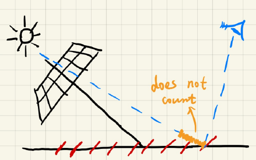
提前需要说明的是：在一个像素内部其深度是一个常数，所以在第一趟渲染shadow map时，从光源沿某一个像素的方向看向一个场景，看到的一个位置是覆盖该位置的一个像素所代表的深度，也就相当于这个场景在一个像素所覆盖的区域内都是一个常数深度，即shadow map将这样一个场景离散成了一系列小片拼成的场景（如上图红色），由于这个深度是从光源看向场景得到的，所以这些红色的小片与光源方向垂直。

对于上图这样一个平面场景来讲，在第一趟渲染中，从光源沿A点方向看向这个场景中的平面，理应能看到点A，但是由于shadow map将这样一个平面的场景离散成了一系列小片形成的场景，而被橙色的小片所遮挡，则shadow map上记录的是到点B的深度；

那么在第二趟从摄像机看向场景的渲染中，对于同一个点A却可以看到，再将A点连回光源处得到A点深度，但是在第一趟渲染shadow map时，这个方向上却被记录了光源到B点的深度，两趟的深度结果就不一致，导致点A处被认为是被遮挡的状态，导致了自遮挡问题的发生。

根据以上理论，在光源垂直于场景平面照射的时候，问题是最小的，而平行于场景平面照射，问题是最大的。

（2）、Adding a (variable) bias to reduce self occlusion

​ –But introducing detached shadow issue

我们可以让两次渲染得到的深度值在比较的时候有一个宽容度，差别在某个范围内则认为是相等。由于光源垂直于平面的时候问题最小，那么这时候宽容度可以比较低，而光源平行于场景的时候问题最大，这时候宽容度可以比较高，通过光源与平面的夹角去动态地调整这个宽容度。

但是这样得到的结果依然出现了问题。由于鞋跟处宽容度还是太大，而丢失了原本该有的遮挡。

（3）、Second-depth shadow mapping

​ –Using the midpoint between first and second depths in SM

​ –Unfortunately, requires objects to be watertight

​ –And the overhead may not worth it

在这种方法里，在第一趟生成shadow map时，我们不仅存最小深度，还存次小深度。假设光从上往下照（如上图），那么最小深度就如左图所示，次小深度如中图所示。用最小深度和次小深度的中间深度作为shadow map来和第二趟的深度值比较。

但是其问题是任何模型都要有正反面，就算是一张纸都要做成一个很薄的box。

而且实现保留最小和次小深度本身也不容易，假设有这样一个可以计算的算法，则其输入是一系列无序的数，而始终要保持最小和次小，最小的很好比较，每次跟输入的值比较即可，但是涉及到最小和次小同时比较就要比较很多次。（虽然时间复杂度还是O(n)，但是RTR does not trust in COMPLEXITY，实时渲染不相信复杂度，只相信绝对的速度）

（4）、Aliasing

由于shadow map上每个像素都可以理解成一个小片，投影出来的阴影图还会涉及到分辨率等问题，所以会出现锯齿。

二、The math behind shadow mapping

1、Inequalities in Calculus

There are a lot of useful inequalities in calculus

2、Approximation in RTR

• But in RTR, we care more about “approximately equal”
• An important approximation throughout RTR

在实时渲染中我们更关心近似相等，在一系列条件下让不等变成约等。

3、In Shadow Mapping

• Recall: the rendering equation with explicit visibility

• Approximated as

用刚刚的公式可以将渲染方程中的V拿出来做归一化。

这时左边是visibility部分，右边是shading部分，并且两者相乘，这正是shadow map的思路

When is it accurate?

​ –Small support

​ (point / directional lighting)

当积分限很小的时候，即小成一个很小很小的点（△），这个式子是准的，也就是当光源是点光源和方向光源时，这个式子没有问题。

​ –Smooth integrand

​ (diffuse bsdf / constant radiance area lighting)

当光照L不变，对应一个面光源（积分限是光源所对应的立体角上），面光源内部的radiance都不变，这里我们就可以认为L是完全smooth的，对于shading point，如果BRDF是diffuse的时候是smooth的。

因此当一个光源是面光源且shading point是diffuse时，这时我们也认为得到的结果是准确的。

三、Percentage closer soft shadows

From Hard Shadows to Soft Shadows

软阴影是从本影到没有阴影之间有一个半影区域，在这些区域看向光源，光源会被部分遮挡。

1、Percentage Closer Filtering (PCF)

• Provides anti-aliasing at shadows’ edges

  ​ –Not for soft shadows (PCSS is, introducing later)

  ​ –Filtering the results of shadow comparisons

PCF是用来做抗锯齿（反走样），但是后来人们发现这个技术还可以做软阴影，于是有了PCSS

• Why not filtering the shadow map?

  ​ –Texture filtering just averages color components, i.e. you’ll get blurred shadow map first

  ​ –Averaging depth values, then comparing, you still get a binary visibility

PCSS不是对渲染出来的阴影图做软阴影处理，也不是对shadow map做处理，而是在阴影判断的时候就做处理（类似于GAMES101中提到的做反走样的流程）

• Solution [Reeves, SIGGARPH 87]

  –Perform multiple (e.g. 7×7) depth comparisons for each fragment

  –Then, averages results of comparisons

  之前判断任何一个点在不在阴影里的时候，我们将shading point连向light算出深度去跟shadow map对应的这点的深度去比较。

  在PCF的算法中，对于一个shading point，依然判断是否落在阴影里，但是投影到light之后不只是找shadow map对应点的像素，同时找shadow map对应该点的像素周围一圈的像素（如7×7），将这一圈的每一个像素深度值都与该shading point深度值去比较，由于每一次比较之后返回的值仅为0和1，做完比较之后把这值取平均，返回到这个点上。

  

  –e.g. for point P on the floor,
  
  (1) compare its depth with all pixels in the red box, e.g. 3×3

  首先将shading point的点P深度值与shadow map中对应该像素以及周围3×3的每一个像素的深度值分别比较

  (2) get the compared results, e.g.

  ​ 1, 0, 1,
  
  ​ 1, 0, 1,
  
  ​ 1, 1, 0,

  然后得到一组返回值

  (3) take avg. to get visibility, e.g. 0.667

  将这组返回值取平均返回给点P

• Does filtering size matter?

  –Small -> sharper

  –Large -> softer

  如果卷积盒取小了边缘会很锐利，锯齿问题不会得到改善，卷积盒取大了虽然锯齿没了，但是图片也糊了。

• Can we use PCF to achieve soft shadow effects?

  软阴影的操作就可以通过对硬阴影取一个很大的卷积盒（filter）来实现

• Key thoughts

  –From hard shadows to soft shadows

  –What’s the correct size to filter?

  –Is it uniform?

2、Percentage Closer Soft Shadows

• Key observation [Fernando et al.]

  –Where is sharper? Where is softer?

物体离投影平面越近，则阴影越硬，离投影平面越远，则阴影越软。

• Key conclusion

  –Filter size <-> blocker distance

  –More accurately, relative average projected blocker depth!

  

  如上图，黄色的W是光源，中间的绿色点是投影物体（遮挡物），灰色W是软阴影区域，两个W及其连线组成了一对相似三角形，根据相似三角形原理可以求出软阴影区域W
  
  _Penumbr
  
  。这个图可以很好地表明物体离投影平面越近，则阴影越硬，离投影平面越远，则阴影越软。

• A mathematical “translation”

根据相似三角形将其软阴影用式子表示出来。

• Now the only question:

  –What’s the blocker depth dBlocker

  卷积盒filter的大小取决于Light的大小和Blocker的大小。由于Blocker可能是很多不规则物体组成的，因此该处的Blocker要取平均：对于一个shading point来说，在一定的范围内，有多少可以在shadow map上挡住其的像素，这些像素记录的深度的平均值是多少。

• The complete algorithm of PCSS

  –Step 1: Blocker search
  
  (getting the average blocker depth in a certain region)

  –Step 2: Penumbra estimation
  
  (use the average blocker depth to determine filter size)

  –Step 3: Percentage Closer Filtering

• Which region to perform blocker search?

  –Can be set constant (e.g. 5×5), but can be better with heuristics

在shading point中，原本就是为了决定在一个shadow map周围多大的范围（filte）做PCF，为了知道这个信息，首先要知道average blocker depth是多少，为了知道这个信息，首先也应该先取一个区域去找average Blocker然后求depth，人们通常一开始固定一个范围大小（如5×5），另外还有更好的方法：

• Which region (on the shadow map) to perform blocker search?

​ –depends on the light size

​ –and receiver’s distance from the light

将shading point连向Light，就可以得到其在shadow map上的区域（如上图红色部分），通过这部分区域来确定filter。