这一部分,我们可以通过实现一个线图神经网络(
LGNN
)来解决
社团检测
。社团检测,或者说图聚类,指的是将图中的节点划分为簇,而且簇内的节点比簇间的节点具有更高的相似性。
在
图神经网络中
,我们可以了解到如何以一种半监督方式来对一张输入图的节点进行分类。我们使用图卷积网络作为图特征的嵌入机制。
为了将图神经网络概况为有监督的社团检测, 论文
Supervised Community Detection with Line Graph Neural Networks.
引入一种基于线图的GNN的变体。该模型的一大亮点是增强了简单的GNN结构,所以它可以在基于非回溯操作定义的线图的邻接边上进行操作。
一个线图神经网络(LGNN)展示了DGL如何通过混合基础张量操作、稀疏矩阵乘法以及消息传递APIs来实现高级的图算法。
下面将介绍社团检测、线图、LGNN及其实现。
Cora数据集上的监督社团检测任务
社团检测
在一个社团检测任务中,我们需要做的是将相似的节点进行聚类,而不是给它们贴上标签。典型的节点相似性被描述为每个类内具有较高的密度。
社团检测和节点分类的区别是什么?与节点分类相比,社团检测强调的是从图上检索聚类信息,而不是给每个节点指派特定的标签。例如,只要一个节点和它的社团成员被聚为一类,那么这个节点属于“社团A”还是“社团B”并不重要,尽管在电影网络分类任务中,把所有“好电影”贴上“烂电影”的标签将是一场灾难。
那么,社区检测算法与其他聚类算法(如k-means)之间的区别是什么呢?社区检测算法作用于图结构数据。与k-means相比,社区检测利用了图结构,而不是简单地根据节点的特性进行集群化。
Cora数据集
Cora是一个科学出版物数据库,有2708篇论文属于七个不同的机器学习领域。这里将Cora表示为一个有向图,每个节点是一篇论文,每个边是一个引用链接(a ->B表示a引用B)。
Cora包含7个类,下面的统计表明,每个类都满足我们对community的假设,即相同类的节点之间的连接概率要高于不同类的节点之间的连接概率。下面的代码片段验证了类内的边比类间的多。
import torch as th
import torch.nn as nn
import torch.nn.functional as F
import dgl
from dgl.data import citation_graph as citegrh

data = citegrh.load_cora()

G = dgl.DGLGraph(data.graph)
labels = th.tensor(data.labels)

# find all the nodes labeled with class 0
label0_nodes = th.nonzero(labels == 0).squeeze()
# find all the edges pointing to class 0 nodes
src, _ = G.in_edges(label0_nodes)
src_labels = labels[src]
# find all the edges whose both endpoints are in class 0
intra_src = th.nonzero(src_labels == 0)
print('Intra-class edges percent: %.4f' % (len(intra_src) / len(src_labels)))
Out:
Intra-class edges percent: 0.7680
带有测试集的Cora数据集的二分类社团子图
为了不失一般性,这里限制任务范围为二分类社团检测。
注意:
为了从Cora中创建一个实际的二分类社团数据集,首先需要从原始的Cora的7各个类提取所有两个类对。对于每一对类,我们需要将一类看作一个社团,并且找到至少包含一条社团间边的最大子图作为训练示例。结果,在这个小的数据集中共有21个训练样本。
下面的代码显示了如何可视化其中一个训练样本及其社团结构。
import networkx as nx
import matplotlib.pyplot as plt

train_set = dgl.data.CoraBinary()
G1, pmpd1, label1 = train_set[1]
nx_G1 = G1.to_networkx()

def visualize(labels, g):
	pos = nx.spring_layout(g, seed=1)
	plt.figure(figsize=(8, 8))
	plt.axis('off')
	nx.draw_networkx(g, pos=pos, node_size=50, cmap=plt.get_cmap('coolwarm'), node_color=labels, edge_color='k', arrows=False, width=0.5, style='dotted', with_labels=False)
visualize(label1, nx_G1)

原文中给出了如何可视化多个社团的例子。
有监督的社团检测
有监督和无监督的方法都可以做到社团检测。在监督方式下,社团检测的公式化见下:
-
每个训练示例包括
(G
,
L
)
(G, L)
(
G
,
L
)
,其中
GG
G
是一个有向图
(V
,
E
)
(V, E)
(
V
,
E
)
。对于V中的每个节点
vv
v
,我们指定一个真实的社团标签
zv
∈
(
0
,
1
)
z_v\in(0, 1)
z
v
∈
(
0
,
1
)
。 -
参数模型
KaTeX parse error: Undefined control sequence: \seta at position 6: f(G, \̲s̲e̲t̲a̲)
对
VV
V
中的所有节点预测标签集合
z~
=
f
(
G
)
\tilde{z}=f(G)
z
~
=
f
(
G
)
。 -
对每个示例
(G
,
L
)
(G, L)
(
G
,
L
)
,模型通过学习来最小化一个专门设计的损失函数
Le
q
u
i
v
a
r
i
a
n
t
=
(
Z
~
,
Z
)
L_{equivariant} =(\tilde{Z}, Z)
L
e
q
u
i
v
a
r
i
a
n
t
=
(
Z
~
,
Z
)
。
注意:
在有监督的设定中,模型会对每个社团预测一个标签。然而, 社团的指定应该等价于标签的排列。为了做到这一点,在每个前向传播过程中,我们选取所有可能标签排列所得到的最小的损失。
数学上,这意味着
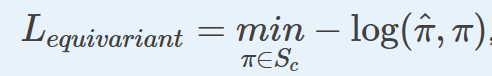
其中,
S
c
S_c
S
c
是标签排列的集合,
π
^
\hat{\pi}
π
^
表示预测标签的集合,
−
log
(
π
^
,
π
)
-\log(\hat{\pi}, \pi)
−
lo
g
(
π
^
,
π
)
指的是负的对数概率。
例如,对于也个样本图,其节点有
1
,
2
,
3
,
4
{1, 2, 3, 4}
1
,
2
,
3
,
4
和分配的社团
A
,
A
,
A
,
B
{A, A, A, B}
A
,
A
,
A
,
B
,每个节点的标签
l
∈
(
0
,
1
)
l\in(0, 1)
l
∈
(
0
,
1
)
,所有可能的排列组合为
S
c
S_c
S
c
= {
{0, 0, 0, 1}, {1, 1, 1, 0}}。
LGNN核心思想
这里的关键创新点是使用线图。不同于之前的模型,消息传递不仅在原图上,比如,来自Cora的二分类社团子图,而且作用在与原图对应的线图上。
线图是什么?
图论中,线图是一种编码原图中边邻居结构的图表示。
具体地,一个线图
L
(
G
)
L(G)
L
(
G
)
将原图
G
G
G
中的边转换成节点。

这里,
e
A
:
=
(
i
−
>
j
)
e_A:=(i->j)
e
A
:
=
(
i
−
>
j
)
和
e
B
:
=
(
j
−
>
k
)
e_B:=(j->k)
e
B
:
=
(
j
−
>
k
)
是原图
G
G
G
中的两条边。在线图
G
L
G_L
G
L
中,它们分别对应于节点
v
A
l
v_A^{l}
v
A
l
和
v
B
l
v_B^{l}
v
B
l
。
那么自然的一个问题是,线图中节点是如何连接的?如何连接两条边呢?这里,我们使用下面的连接规则:
l
g
lg
l
g
中两节点
v
A
l
v_A^{l}
v
A
l
和
v
B
l
v_B^{l}
v
B
l
是连接的如果
g
g
g
中对应的两条边
e
A
e_A
e
A
和
e
B
e_B
e
B
共享且只共享一个节点:
e
A
e_A
e
A
的终节点是
e
B
e_B
e
B
的源节点。
注意:
数学上,这个定义对应于称之为非回溯操作的概念:
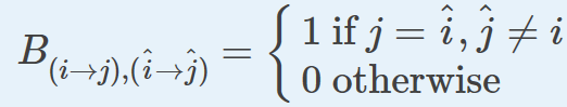
当
B
n
o
d
e
1
,
n
o
d
e
2
=
1
B_{node1, node2} =1
B
n
o
d
e
1
,
n
o
d
e
2
=
1
时,会形成一条边。
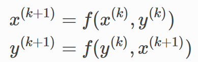
LGNN的一层——算法结构
LGNN将一系列线图神经网路层连在一起。图表示
x
x
x
及其相应的线图
y
y
y
随数据流的变化如下。

在第
k
k
k
层,第
l
l
l
个通道的第
i
i
i
个神经元利用下面的式子更新其嵌入
x
i
,
l
(
k
+
1
)
x_{i, l}^{(k+1)}
x
i
,
l
(
k
+
1
)
:

接下来,线图的表示
y
i
,
l
(
k
+
1
)
y_{i, l}^{(k+1)}
y
i
,
l
(
k
+
1
)
如下:

其中,
s
k
i
p
−
c
o
n
n
e
c
t
i
o
n
skip-connection
s
k
i
p
−
c
o
n
n
e
c
t
i
o
n
指的是执行相同的操作,不包含非线性的
ρ
\rho
ρ
,包含线性映射
用DGL实现LGNN
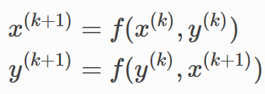
即使上一节中的方程式可能看起来令人生畏,但在实现LGNN之前它有助于理解以下信息。
这两个式子是对称的,可以作为同一类中不同参数的两个实例。第一个式子作用在图表示
x
x
x
上,而第二个式子作用在线图表示
y
y
y
上。我们把这些抽象表示为
f
f
f
。那第一个表示为
f
(
x
,
y
;
θ
x
)
f(x, y; \theta_x)
f
(
x
,
y
;
θ
x
)
,第二个表示为
f
(
y
,
x
,
θ
y
)
f(y, x, \theta_y)
f
(
y
,
x
,
θ
y
)
。即,将它们参数化,以分别计算原图和对应线图的表示。
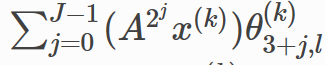
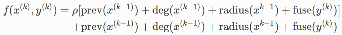
每个式子都包含四项,以第一个为例,后面的类似。
-
x(
k
)
θ
1
,
l
(
k
)
x^{(k)}\theta_{1, l}^{(k)}
x
(
k
)
θ
1
,
l
(
k
)
,是上一层输出
x(
k
)
x^{(k)}
x
(
k
)
的线性映射,表示为
pr
e
v
(
x
)
prev(x)
p
r
e
v
(
x
)
。 -
(D
x
(
k
)
)
θ
2
,
l
(
k
)
(D_x^{(k)})\theta_{2, l}^{(k)}
(
D
x
(
k
)
)
θ
2
,
l
(
k
)
,作用在
x(
k
)
x^{(k)}
x
(
k
)
上的度操作的线性映射,表示为
de
g
(
x
)
deg(x)
d
e
g
(
x
)
。 -
作用于
x(
k
)
x^{(k)}
x
(
k
)
上的
2j
2^j
2
j
的邻接操作的和,表示为
ra
d
i
u
s
(
x
)
radius(x)
r
a
d
i
u
s
(
x
)
。 -
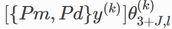
使用关联矩阵{
Pm
,
P
d
P_m, P_d
P
m
,
P
d
}融合另一个图的嵌入信息,然后加上一个线性映射,表示为
fu
s
e
(
y
)
fuse(y)
f
u
s
e
(
y
)
。
每一项都会用不同的参数多次计算,并且在求和之后不再进行非线性化。因此,
f
f
f
可以写成:
两个式子通过下面的顺序连接:
注意:
通过下面的解释,你可以对{
P
m
,
P
d
P_m, P_d
P
m
,
P
d
}有更为透彻的理解。大概地讲,就是在循环简单的传递中,
g
g
g
和
l
g
lg
l
g
(线图)之间的关系。这里,{
P
m
,
P
d
P_m, P_d
P
m
,
P
d
}可作为数据集中的SciPy COO稀疏矩阵来完成,并在分批时将它们堆叠为张量。另一种分批的方法是把{
P
m
,
P
d
P_m, P_d
P
m
,
P
d
}看作二部图的邻接矩阵,它实现了从线图特征到图的映射,反之亦然。
实现
p
r
e
v
prev
p
r
e
v
和
d
e
g
deg
d
e
g
的张量操作
线性映射和度操作都只是简单的矩阵乘法。将它们写成PyTorch的张量操作。
在__init__中,定义映射变量。
self.linear_prev = nn.Linear(in_feats, out_feats)
self.linear_deg = nn.Linear(in_feats, out_feats)
在forward()中,
p
r
e
v
prev
p
r
e
v
和
d
e
g
deg
d
e
g
同其它PyTorch的张量操作一样。
prev_proj = self.linear_prev(feat_a)
prev_proj = self.linear_deg(deg * feat_a)
DGL中实现
r
a
d
i
u
s
radius
r
a
d
i
u
s
作为消息传递
正如GCN中提到的,我们可以形成一个邻接算子作为一步的消息传递。作为推广,
2
j
2^j
2
j
邻接操作可以通过执行
2
j
2^j
2
j
步消息传递来做到。因此,其和等同于
2
j
2^j
2
j
个节点表示的和,
j
=
0
,
1
,
2..
j=0, 1, 2..
j
=
0
,
1
,
2
.
.
步消息传递。
在__init__中,定义用在
2
j
2^j
2
j
步消息传递的映射变量。
self.linear_radius = nn.ModuleList([nn.Linear(in_feats, out_feats) for i in range(radius)])
在__forward__中,使用下面的函数aggregate_radius()来聚合多跳的数据。注意update_all被调用多次。
# Return a list containing features gathered from multiple radius.
import dgl.function as fn
def aggregate_radius(radius, g, z):
	# initializing list to collect message passing result
	z_list = []
	g.ndata['z'] = z
	# pulling message from 1-hop neighbourhood
	g.update_all(fn.copy_src(src='z', out='m'), fn.sum(msg='m', out='z'))
	z_list.append(g.ndata['z'])
	for i in range(radius - 1):
		for j in range(2 ** i):
			# pulling message from 2^j neighborhood
			g.update_all(fn.copy_src(src='z', out='m'), fn.sum(msg='m', out='z'))
	z_list.append(g.ndata['z'])
	return z_list
实现
f
u
s
e
fuse
f
u
s
e
作为稀疏矩阵乘法
{
P
m
,
P
d
P_m, P_d
P
m
,
P
d
}是一个每列只有两个非零输入的稀疏矩阵。因此,我们可以将其构建为数据集中的一个稀疏矩阵,并通过稀疏矩阵乘法来实现
f
u
s
e
fuse
f
u
s
e
。
在__forward__中:
fuse = self.linear_fuse(th.mm(pm_pd, feat_b))
f
(
x
,
y
)
f(x, y)
f
(
x
,
y
)
的完成
最后,下面展示了如何将这些项加起来,并将它传递给skip connection和batch norm。
result = prev_proj + deg_proj + radius_proj + fuse
传递结果到skip connection。
result = th.cat([result[:, :n], F.relu(result[:, n:])], 1)
然后将结果传递给batch norm。
result = self.bn(result) # Batch Normalization
这里是一个LGNN层的提取
f
(
x
,
y
)
f(x, y)
f
(
x
,
y
)
的完整代码。
class LGNNCore(nn.Module):
    def __init__(self, in_feats, out_feats, radius):
        super(LGNNCore, self).__init__()
        self.out_feats = out_feats
        self.radius = radius

        self.linear_prev = nn.Linear(in_feats, out_feats)
        self.linear_deg = nn.Linear(in_feats, out_feats)
        self.linear_radius = nn.ModuleList(
                [nn.Linear(in_feats, out_feats) for i in range(radius)])
        self.linear_fuse = nn.Linear(in_feats, out_feats)
        self.bn = nn.BatchNorm1d(out_feats)

    def forward(self, g, feat_a, feat_b, deg, pm_pd):
        # term "prev"
        prev_proj = self.linear_prev(feat_a)
        # term "deg"
        deg_proj = self.linear_deg(deg * feat_a)

        # term "radius"
        # aggregate 2^j-hop features
        hop2j_list = aggregate_radius(self.radius, g, feat_a)
        # apply linear transformation
        hop2j_list = [linear(x) for linear, x in zip(self.linear_radius, hop2j_list)]
        radius_proj = sum(hop2j_list)

        # term "fuse"
        fuse = self.linear_fuse(th.mm(pm_pd, feat_b))

        # sum them together
        result = prev_proj + deg_proj + radius_proj + fuse

        # skip connection and batch norm
        n = self.out_feats // 2
        result = th.cat([result[:, :n], F.relu(result[:, n:])], 1)
        result = self.bn(result)

        return result
将LGNN的提取连起来作为LGNN的一层
为了实现
示例代码中,将两个LGNNCore实例连起来,在前向传递过程中有不同的参数。
class LGNNLayer(nn.Module):
    def __init__(self, in_feats, out_feats, radius):
        super(LGNNLayer, self).__init__()
        self.g_layer = LGNNCore(in_feats, out_feats, radius)
        self.lg_layer = LGNNCore(in_feats, out_feats, radius)

    def forward(self, g, lg, x, lg_x, deg_g, deg_lg, pm_pd):
        next_x = self.g_layer(g, x, lg_x, deg_g, pm_pd)
        pm_pd_y = th.transpose(pm_pd, 0, 1)
        next_lg_x = self.lg_layer(lg, lg_x, x, deg_lg, pm_pd_y)
        return next_x, next_lg_x
连接LGNN层
用三个隐藏层定义一个LGNN,见下例。
Define an LGNN with three hidden layers, as in the following example.
class LGNN(nn.Module):
    def __init__(self, radius):
        super(LGNN, self).__init__()
        self.layer1 = LGNNLayer(1, 16, radius)  # input is scalar feature
        self.layer2 = LGNNLayer(16, 16, radius)  # hidden size is 16
        self.layer3 = LGNNLayer(16, 16, radius)
        self.linear = nn.Linear(16, 2)  # predice two classes

    def forward(self, g, lg, pm_pd):
        # compute the degrees
        deg_g = g.in_degrees().float().unsqueeze(1)
        deg_lg = lg.in_degrees().float().unsqueeze(1)
        # use degree as the input feature
        x, lg_x = deg_g, deg_lg
        x, lg_x = self.layer1(g, lg, x, lg_x, deg_g, deg_lg, pm_pd)
        x, lg_x = self.layer2(g, lg, x, lg_x, deg_g, deg_lg, pm_pd)
        x, lg_x = self.layer3(g, lg, x, lg_x, deg_g, deg_lg, pm_pd)
        return self.linear(x)
训练和预测
首先加载数据。
from torch.utils.data import DataLoader
training_loader = DataLoader(train_set, batch_size=1, collate_fn=train_set.collate_fn, drop_last=True)
然后定义主训练循环。注意到每个训练样本包含三个对象:一个DGLGraph,一个SciPy稀疏矩阵和一个numpy.ndarray的标签数组。使用下面的命令来创建线图:
lg = g.line_graph(backtracking=False)
注意到backtracking=False是为了正确模拟非回溯操作。我们也定义了一个通用函数来转换SciPy稀疏矩阵为torch稀疏张量。
# Create the model
model = LGNN(radius=3)
# define the optimizer
optimizer = th.optim.Adam(model.parameters(), lr=1e-2)

# A utility function to convert a scipy.coo_matrix to torch.SparseFloat
def sparse2th(mat):
    value = mat.data
    indices = th.LongTensor([mat.row, mat.col])
    tensor = th.sparse.FloatTensor(indices, th.from_numpy(value).float(), mat.shape)
    return tensor

# Train for 20 epochs
for i in range(20):
    all_loss = []
    all_acc = []
    for [g, pmpd, label] in training_loader:
        # Generate the line graph.
        lg = g.line_graph(backtracking=False)
        # Create torch tensors
        pmpd = sparse2th(pmpd)
        label = th.from_numpy(label)

        # Forward
        z = model(g, lg, pmpd)

        # Calculate loss:
        # Since there are only two communities, there are only two permutations
        #  of the community labels.
        loss_perm1 = F.cross_entropy(z, label)
        loss_perm2 = F.cross_entropy(z, 1 - label)
        loss = th.min(loss_perm1, loss_perm2)

        # Calculate accuracy:
        _, pred = th.max(z, 1)
        acc_perm1 = (pred == label).float().mean()
        acc_perm2 = (pred == 1 - label).float().mean()
        acc = th.max(acc_perm1, acc_perm2)
        all_loss.append(loss.item())
        all_acc.append(acc.item())

        optimizer.zero_grad()
        loss.backward()
        optimizer.step()

    niters = len(all_loss)
    print("Epoch %d | loss %.4f | accuracy %.4f" % (i,
        sum(all_loss) / niters, sum(all_acc) / niters))
Out:
Epoch 0 | loss 0.5751 | accuracy 0.6873
Epoch 1 | loss 0.5025 | accuracy 0.7742
Epoch 2 | loss 0.5078 | accuracy 0.7551
Epoch 3 | loss 0.4895 | accuracy 0.7624
Epoch 4 | loss 0.4682 | accuracy 0.7910
Epoch 5 | loss 0.4461 | accuracy 0.7992
Epoch 6 | loss 0.4815 | accuracy 0.7838
Epoch 7 | loss 0.4542 | accuracy 0.7970
Epoch 8 | loss 0.4338 | accuracy 0.8172
Epoch 9 | loss 0.4694 | accuracy 0.7604
Epoch 10 | loss 0.4525 | accuracy 0.7958
Epoch 11 | loss 0.4388 | accuracy 0.7941
Epoch 12 | loss 0.4440 | accuracy 0.8092
Epoch 13 | loss 0.4325 | accuracy 0.7982
Epoch 14 | loss 0.4087 | accuracy 0.8137
Epoch 15 | loss 0.4073 | accuracy 0.8129
Epoch 16 | loss 0.4123 | accuracy 0.8133
Epoch 17 | loss 0.4061 | accuracy 0.8201
Epoch 18 | loss 0.4100 | accuracy 0.8123
Epoch 19 | loss 0.4170 | accuracy 0.8348
可视化训练过程
pmpd1 = sparse2th(pmpd1)
LG1 = G1.line_graph(backtracking=False)
z = model(G1, LG1, pmpd1)
_, pred = th.max(z, 1)
visualize(pred, nx_G1)
visualize(label1, nx_G1)
对图进行分批并行处理
LGNN选择不同图的集合,分批可以用作并行。
批处理可以由数据加载器本身做的。 在PyTorch数据加载器的collate_fn中,使用DGL的batched_graph API对图进行批处理。 DGL通过将图合并成一个大图来对图进行批处理,每个较小图的邻接矩阵都是沿着大图邻接矩阵对角线的一个块。 将数学中{Pm,Pd}连接为块对角线矩阵,对应于DGL批处理图API。
def collate_fn(batch):
    graphs, pmpds, labels = zip(*batch)
    batched_graphs = dgl.batch(graphs)
    batched_pmpds = sp.block_diag(pmpds)
    batched_labels = np.concatenate(labels, axis=0)
    return batched_graphs, batched_pmpds, batched_labels