贝叶斯滤波
1. 概率基础回顾
条件概率:
p
(
x
∣
y
)
=
p
(
x
,
y
)
/
p
(
y
)
p
(
x
,
y
)
=
p
(
x
∣
y
)
p
(
y
)
=
p
(
y
∣
x
)
p
(
x
)
p(x|y)=p(x,y)/p(y) \\ \ \\ p(x,y)=p(x|y)p(y)=p(y|x)p(x)
p
(
x
∣
y
)
=
p
(
x
,
y
)
/
p
(
y
)
p
(
x
,
y
)
=
p
(
x
∣
y
)
p
(
y
)
=
p
(
y
∣
x
)
p
(
x
)
全概率公式:
p
(
x
)
=
∑
y
p
(
x
,
y
)
=
∑
y
p
(
x
∣
y
)
p
(
y
)
p(x) = \sum\limits_y {p(x,y)}=\sum\limits_y {p(x|y)p(y)}
p
(
x
)
=
y
∑
p
(
x
,
y
)
=
y
∑
p
(
x
∣
y
)
p
(
y
)
全概率公式的意义在于,当某一事件的概率难以求得时,可转化为在一系列条件下发生概率的和。
2. 贝叶斯公式
2.1 贝叶斯公式
基于条件概率公式和全概率公式,我们可以导出贝叶斯公式:
$$
\begin{array}{c} P(x,y) = P(x|y)P(y) = P(y|x)P(x)\
\Rightarrow \
\end{array}
$$
P
(
x
∣
y
)
=
P
(
y
∣
x
)
P
(
x
)
P
(
y
)
=
P
(
y
∣
x
)
P
(
x
)
∑
y
p
(
x
∣
y
)
p
(
y
)
P(x\,\left| {\,y} \right.) = \frac{
{P(y|x)\,\,P(x)}}{
{P(y)}} = \frac {
{P(y|x)\,\,P(x)}} {
{ \sum\limits_y {p(x|y)p(y)} }}
P
(
x
∣
y
)
=
P
(
y
)
P
(
y
∣
x
)
P
(
x
)
=
y
∑
p
(
x
∣
y
)
p
(
y
)
P
(
y
∣
x
)
P
(
x
)
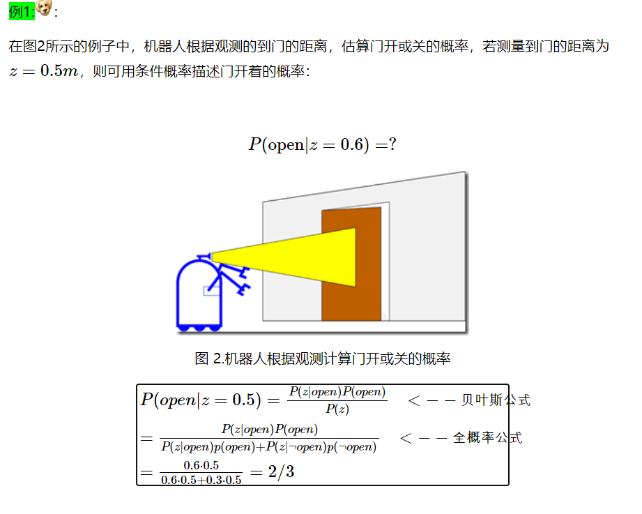
- 这里x是某种状态,y 是某种预观测。下面例子中 x 代表门开关,y 代表距离z
-
我们称P(y|x)为
causal knowledge(因果知识)
,意即由x的已知情况,就可以推算y发生的概率,例如在图2的例子中,已知如果门开着,则z=0.5m的概率为0.6;如果门关着,则z=0.5m的的概率为0.3。 -
P(x) 为
prior knowledge
,先验概率。可以设开关概率都是 0.5。 -
P(x|y) 是基于观测对状态的诊断或推断。
贝叶斯公式的本质就是利用causal knowledge和prior knowledge来进行状态推断或推理
2.2 贝叶斯公式的计算
可以把分母项看成归一化系数
η
\eta
η
P
(
x
∣
y
)
=
P
(
y
∣
x
)
P
(
x
)
P
(
y
)
=
η
P
(
y
∣
x
)
P
(
x
)
η
=
P
(
y
)
−
1
=
1
∑
x
P
(
y
∣
x
)
P
(
x
)
\begin{array}{l} P(x\,\left| {\,y} \right.) = \frac{
{P(y|x)\,\,P(x)}}{
{P(y)}} = \eta \;P(y|x)\,P(x)\\ \eta = P{(y)^{ – 1}} = \frac{1}{
{\sum\limits_x {P(y|x)} P(x)}} \end{array}
P
(
x
∣
y
)
=
P
(
y
)
P
(
y
∣
x
)
P
(
x
)
=
η
P
(
y
∣
x
)
P
(
x
)
η
=
P
(
y
)
−
1
=
x
∑
P
(
y
∣
x
)
P
(
x
)
1
Algorithm:
∀
x
:
a
u
x
x
∣
y
=
P
(
y
∣
x
)
P
(
x
)
η
=
1
∑
x
a
u
x
x
∣
y
∀
x
:
P
(
x
∣
y
)
=
η
a
u
x
x
∣
y
\begin{array}{l} \forall x:{\rm{au}}{
{\rm{x}}_{x|y}} = P(y|x)\,\,P(x)\\ \eta = \frac{1}{
{\sum\limits_x {
{\rm{au}}{
{\rm{x}}_{x|y}}} }}\\ \forall x:P(x|y) = \eta \;{\rm{au}}{
{\rm{x}}_{x|y}} \end{array}
∀
x
:
a
u
x
x
∣
y
=
P
(
y
∣
x
)
P
(
x
)
η
=
x
∑
a
u
x
x
∣
y
1
∀
x
:
P
(
x
∣
y
)
=
η
a
u
x
x
∣
y
2.3 贝叶斯公式融合多种观测
P
(
x
∣
y
,
z
)
=
P
(
x
,
y
,
z
)
P
(
y
,
z
)
=
P
(
y
∣
x
,
z
)
p
(
x
,
z
)
P
(
y
,
z
)
=
P
(
y
∣
x
,
z
)
p
(
x
∣
z
)
p
(
z
)
P
(
y
∣
z
)
p
(
z
)
=
P
(
y
∣
x
,
z
)
p
(
x
∣
z
)
P
(
y
∣
z
)
\begin{array}{l} P(x|y,z){\rm{ = }}\frac{
{P(x,y,z)}}{
{P(y,z)}}\\ = \frac{
{P(y|x,z)p(x,z)}}{
{P(y,z)}}\\ = \frac{
{P(y|x,z)p(x|z)p(z)}}{
{P(y|z)p(z)}}\\ = \frac{
{P(y|x,z)p(x|z)}}{
{P(y|z)}} \end{array}
P
(
x
∣
y
,
z
)
=
P
(
y
,
z
)
P
(
x
,
y
,
z
)
=
P
(
y
,
z
)
P
(
y
∣
x
,
z
)
p
(
x
,
z
)
=
P
(
y
∣
z
)
p
(
z
)
P
(
y
∣
x
,
z
)
p
(
x
∣
z
)
p
(
z
)
=
P
(
y
∣
z
)
P
(
y
∣
x
,
z
)
p
(
x
∣
z
)
所以,在预观测 y, z 条件下 x 发生的概率:
P
(
x
∣
y
,
z
)
=
P
(
y
∣
x
,
z
)
P
(
x
∣
z
)
P
(
y
∣
z
)
P(x|y,z) = \frac{
{P(y|x,z)\,\,P(x|z)}}{
{P(y|z)}}
P
(
x
∣
y
,
z
)
=
P
(
y
∣
z
)
P
(
y
∣
x
,
z
)
P
(
x
∣
z
)
2.4 贝叶斯递推公式
由此,我们来推导贝叶斯滤波的递推公式:
P
(
x
∣
z
1
,
…
,
z
n
)
=
?
P(x|z_1, \ldots ,z_n) =?
P
(
x
∣
z
1
,
…
,
z
n
)
=
?
再由Markov属性,在x已知的情况下,
z
n
z_n
z
n
同
{
z
n
−
1
,
…
,
z
1
}
\{ z_{n-1}, \ldots, z_1 \}
{
z
n
−
1
,
…
,
z
1
}
无关
P
(
x
∣
z
1
,
…
,
z
n
)
=
P
(
z
n
∣
x
,
z
1
,
…
,
z
n
–
1
)
P
(
x
∣
z
1
,
…
,
z
n
–
1
)
P
(
z
n
∣
z
1
,
…
,
z
n
–
1
)
=
P
(
z
n
∣
x
)
P
(
x
∣
z
1
,
…
,
z
n
–
1
)
P
(
z
n
∣
z
1
,
…
,
z
n
–
1
)
\begin{array}{c} P(x|z_1, \ldots ,z_n) = \frac{
{P(z_n|x,z_1, \ldots ,z_{n – 1})\;P(x|z1, \ldots ,z_{n – 1})}}{
{P(z_n|z_1, \ldots ,z_{n – 1})}}\\ =\frac{
{P(z_n|x)\;P(x|z1, \ldots ,z_{n – 1})}}{
{P(z_n|z_1, \ldots ,z_{n – 1})}} \end{array}
P
(
x
∣
z
1
,
…
,
z
n
)
=
P
(
z
n
∣
z
1
,
…
,
z
n
–
1
)
P
(
z
n
∣
x
,
z
1
,
…
,
z
n
–
1
)
P
(
x
∣
z
1
,
…
,
z
n
–
1
)
=
P
(
z
n
∣
z
1
,
…
,
z
n
–
1
)
P
(
z
n
∣
x
)
P
(
x
∣
z
1
,
…
,
z
n
–
1
)
所以:
$$
\begin{array}{*{20}{l}}
{P(x|{z_1}, \ldots ,{z_n})}&{ = \frac{
{P({z_n}|x);P(x|{z_1}, \ldots ,{z_{n{\rm{ – }}1}})}}{
{P({z_n}|{z_1}, \ldots ,{z_{n – 1}})}}}\ {}&{ = {\eta
n};P({z_n}|x);P(x|{z_1}, \ldots ,{z
{n – 1}})}\
{}&\begin{array}{l} = {\eta
n};P({z_n}|x);{\eta
{n – 1}}P({z
{n – 1}}|x)P(x|{z_1}, \ldots ,{z
{n – 2}})\ = {\eta _1} \cdots {\eta
n};\prod\limits
{i = 1…n} {P({z_i}|x)} ;P(x)
\end{array}
\end{array}
$$
3. 如何融入动作
在实际问题中,对象总是处在一个动态变化的环境中,例如:
- 机器人自身的动作影响了环境状态
- 其它对象,比如人的动作影响了环境状态
- 或者就是简单的环境状态随着时间发生了变化。
如何在Bayes模型中来描述动作的影响呢?
- 首先,动作所带来的影响也总是具有不确定性的
- 其次,相比于观测,动作一般会使得对象的状态更为模糊(或更不确定)。
我们用u来描述动作,在 x’ 状态下,执行动作 u 后,对象状态变成 x 的概率为:
P
(
x
∣
u
,
x
’
)
P(x|u,x’)
P
(
x
∣
u
,
x
’
)
动作对状态的影响一般由状态转移模型来描述。如图3所示,表示了“关门”这个动作对状态影响的转移模型。这个状态转移模型表示:关门这个动作有0.1的失败概率,所以当门是open状态时,执行“关门”动作,门有0.9的概率转为closed状态,有0.1的概率保持在open状态。门是closed的状态下,执行“关门”动作,门仍然是关着的。
执行某一动作后,计算动作后的状态概率,需要考虑动作之前的各种状态情况,把所有情况用全概率公式计算:
-
连续情况下
P(
x
∣
u
)
=
∫
P
(
x
∣
u
,
x
′
)
P
(
x
′
)
d
x
′
P(x|u) = \int {P(x|u,x’)P(x’)dx’}
P
(
x
∣
u
)
=
∫
P
(
x
∣
u
,
x
′
)
P
(
x
′
)
d
x
′
-
离散情况下
P(
x
∣
u
)
=
∑
P
(
x
∣
u
,
x
′
)
P
(
x
′
)
P(x|u) = \sum {P(x|u,x’)P(x’)}
P
(
x
∣
u
)
=
∑
P
(
x
∣
u
,
x
′
)
P
(
x
′
)
例3:

在例2的基础上,如果按照图3所示的状态转移关系,机器人执行了一次关门动作, 计算动作后门开着的概率?
P
(
o
p
e
n
∣
u
)
=
∑
P
(
o
p
e
n
∣
u
,
x
′
)
P
(
x
′
)
=
P
(
o
p
e
n
∣
u
,
o
p
e
n
)
P
(
o
p
e
n
)
+
P
(
o
p
e
n
∣
u
,
c
l
o
s
e
d
)
P
(
c
l
o
s
e
d
)
=
1
10
∗
0.8
+
0
1
∗
0.2
=
0.08
\begin{array}{lllll} P(open|u) & = \sum {P(open|u,x’)P(x’)} \\ & \,\, = P(open|u,open)P(open)\\ & \quad + P(open|u,closed)P(closed)\\ & {\kern 1pt} \; = \frac{1}{
{10}} * 0.8 + \frac{0}{1} * 0.2 = 0.08\\ \end{array}
P
(
o
p
e
n
∣
u
)
=
∑
P
(
o
p
e
n
∣
u
,
x
′
)
P
(
x
′
)
=
P
(
o
p
e
n
∣
u
,
o
p
e
n
)
P
(
o
p
e
n
)
+
P
(
o
p
e
n
∣
u
,
c
l
o
s
e
d
)
P
(
c
l
o
s
e
d
)
=
1
0
1
∗
0
.
8
+
1
0
∗
0
.
2
=
0
.
0
8
P
(
c
l
o
s
e
d
∣
u
)
=
∑
P
(
c
l
o
s
e
d
∣
u
,
x
′
)
P
(
x
′
)
=
P
(
c
l
o
s
e
d
∣
u
,
o
p
e
n
)
P
(
o
p
e
n
)
+
P
(
c
l
o
s
e
d
∣
u
,
c
l
o
s
e
d
)
P
(
c
l
o
s
e
d
)
=
9
10
∗
0.8
+
1
1
∗
0.2
=
0.92
\begin{array}{lllll} P(closed|u) & = \sum {P(closed|u,x’)P(x’)} \\ & \,\, = P(closed|u,open)P(open)\\ & \quad + P(closed|u,closed)P(closed)\\ & {\kern 1pt} \; = \frac{9}{
{10}} * 0.8 + \frac{1}{1} * 0.2 = 0.92 \end{array}
P
(
c
l
o
s
e
d
∣
u
)
=
∑
P
(
c
l
o
s
e
d
∣
u
,
x
′
)
P
(
x
′
)
=
P
(
c
l
o
s
e
d
∣
u
,
o
p
e
n
)
P
(
o
p
e
n
)
+
P
(
c
l
o
s
e
d
∣
u
,
c
l
o
s
e
d
)
P
(
c
l
o
s
e
d
)
=
1
0
9
∗
0
.
8
+
1
1
∗
0
.
2
=
0
.
9
2
所以门还开着的概率为 0.08 。
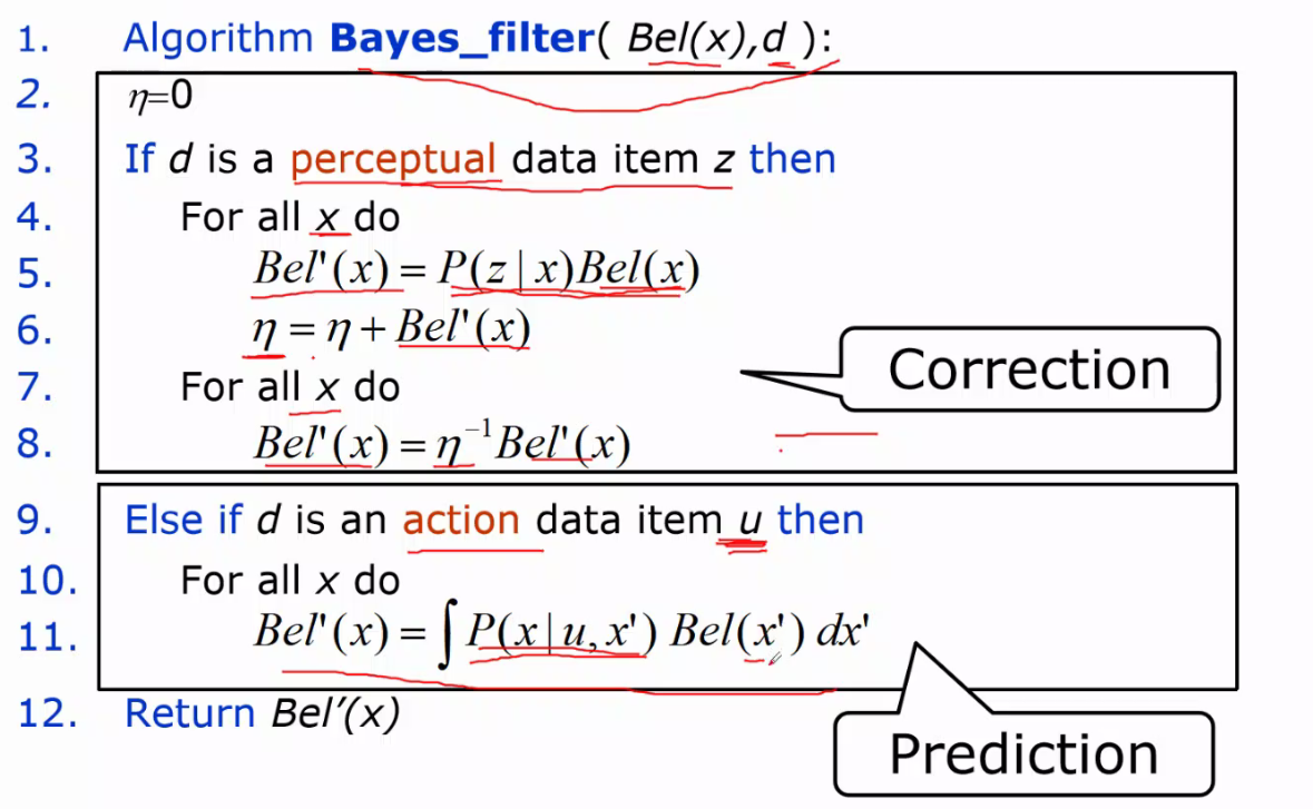
贝叶斯滤波算法
贝叶斯滤波推导:
-
Markov性假设: t 时刻状态仅由 t-1 时刻状态
xt
−
1
x_{t-1}
x
t
−
1
以及t时刻动作
ut
u_{t}
u
t
决定,t时刻观测仅由 t 时刻状态决定。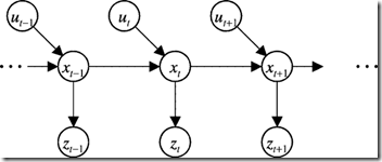
-
静态环境,即对象周边的环境假设是不变的
-
观测噪声、模型噪声等是相互独立的
推导过程:
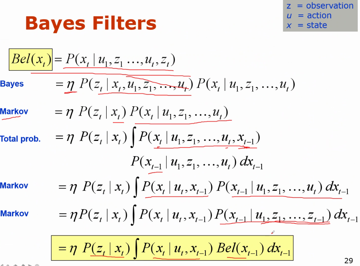
η
\eta
η
是求和的倒数
3.2 贝叶斯滤波算法
由推导可以看出贝叶斯算法两个步骤,第一是基于
x
t
−
1
,
u
t
x_{t-1}, u_t
x
t
−
1
,
u
t
预测
x
t
x_t
x
t
,第二是基于观测
z
t
z_t
z
t
更新状态
x
t
x_t
x
t
。
Bayes algorithm
3.3 多个观测
z
1
,
z
2
,
…
z_1, z_2,\dots
z
1
,
z
2
,
…
可以把每一个观测看作相互独立,对这些观测
依次
更新状态。
贝叶斯滤波matlab程序实现
问题:一个一维空间里,有一个小机器人,可以测量距离前后墙壁的距离(测不准,高斯误差),可以前后移动(移动成功和不成功),用贝叶斯滤波对机器人进行定位。
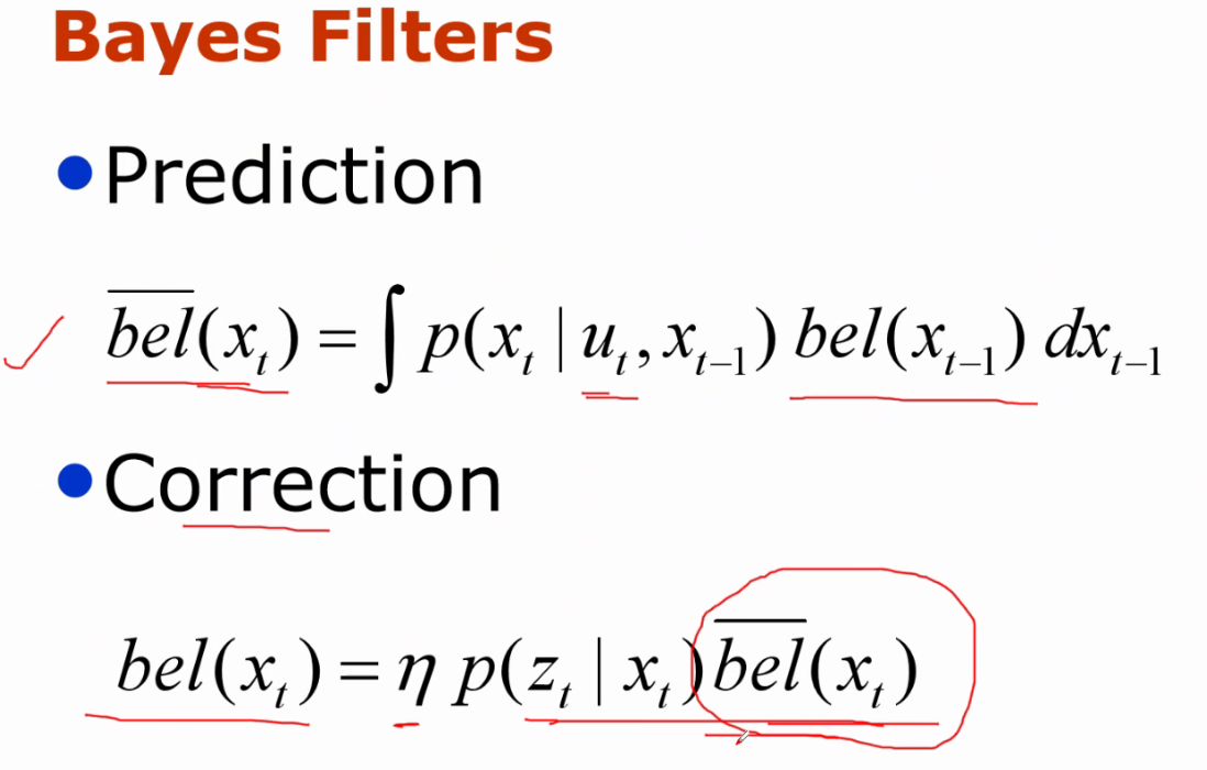
下面是关键函数贝叶斯滤波,主要是实现下面的公式:
对于给定观测:
b
e
l
(
x
t
)
=
η
p
(
z
t
∣
x
t
)
b
e
l
‾
(
x
t
)
{bel}\left(x_{t}\right)=\eta p\left(z_{t} \mid x_{t}\right) \overline{
{bel}}\left(x_{t}\right)
b
e
l
(
x
t
)
=
η
p
(
z
t
∣
x
t
)
b
e
l
(
x
t
)
对于给定动作:
P
(
x
∣
u
)
=
∑
P
(
x
∣
u
,
x
′
)
P
(
x
′
)
P(x|u) = \sum {P(x|u,x’)P(x’)}
P
(
x
∣
u
)
=
∑
P
(
x
∣
u
,
x
′
)
P
(
x
′
)
    function Belief = Bayesian_Filter(Belief,flag,SenseProb,TModel,X)
        n = size(Belief,1);
        if(flag==0) % observation
            %根据S的感知结果,计算感知概率
            disp('receive observation');
            Belief = Belief .* SenseProb(1, :).';
            Belief = Belief ./ sum(Belief);

            Belief = Belief .* SenseProb(2, :).';
            Belief = Belief ./ sum(Belief);

        elseif(flag==1) % action
            disp('receive action 1');
            u=1;
            Belief_update = zeros(n, 1);
            for i1 = X
                tProb = TransitionModel(TModel, i1, u).';
                Belief_temp = Belief .* tProb;
                Belief_update(i1) = sum(Belief_temp);
            end
            Belief = Belief_update;

        elseif(flag==2) % action
            disp('receive action 2');
            u=2;
            Belief_update = zeros(n, 1);
            for i1 = X
                tProb = TransitionModel(TModel, i1, u).';
                Belief_temp = Belief .* tProb;
                Belief_update(i1) = sum(Belief_temp);
            end
            Belief = Belief_update;
        else
            disp('t is invalid');
        end
        disp({'置信度之和应为1:',sum(Belief), '\n真实位置:', groundTruth});
    end
下面是全部代码
function BayesianFilterRobot()
%% Setting up the environment
% Yongcai Wang, ycw@ruc.edu.cn
% 2019-9-20
% A robot is moving along a corridor of 20 meters. X=1:20;
% Two sensors are deployed at the two ends of the corridor. Pos(S)=[0,21];
% The robot moves along the corridor from 1 to 20.
% The motions include moving right, moving left and stand still.

figure;
set(figure(1) ,'KeyPressFcn',@keyhandler,'Name','Bayesian Update');

nGrids = 20;
X=1:nGrids;
Belief=1/nGrids*ones(nGrids,1); %初始化的机器人位置置信度
groundTruth = 1; %机器人的真实位置;

%%两个传感器,分别检测到两端墙的距离,传感器的是0均值,方差为2
Sensor(1)=struct('toWall',0,'Sigma',2)
Sensor(2)=struct('toWall',21,'Sigma',2)

%% 获得传感器的读数
SensorData = TakeSensorReadings(groundTruth);

%% 绘制机器人位置置信度分布
updateWorld(Belief);

%% 定义两种动作的概率转移矩阵
nAction = 2;
TModel = zeros(nAction,nGrids, nGrids);
for i=1:1:nGrids-2
    TModel(1,i,i)=0.1;
    TModel(1,i,i+1)=0.7;
    TModel(1,i,i+2)=0.2;
end
TModel(1,nGrids,nGrids)=1;
TModel(1,nGrids-1,nGrids)=0.9;
TModel(1,nGrids-1,nGrids-1)=0.1;

for i=3:1:nGrids
    TModel(2,i,i)=0.1;
    TModel(2,i,i-1)=0.7;
    TModel(2,i,i-2)=0.2;
end
TModel(2,1,1)=1;
TModel(2,2,1)=0.9;
TModel(2,2,2)=0.1;

disp('start');

%% 响应键盘动作的主函数
    function keyhandler(src,evnt) %#ok<INUSL>
        if strcmp(evnt.Key,'rightarrow')
            SensorData = TakeSensorReadings(groundTruth);
            SenseProb = SensingModel(SensorData, X, Sensor);
            Belief=Bayesian_Filter(Belief,0,SenseProb,TModel,X);
            groundTruth=MoveRight(groundTruth,nGrids);
            Belief=Bayesian_Filter(Belief,1,SenseProb,TModel,X);
            updateWorld(Belief);
        elseif strcmp(evnt.Key,'leftarrow')
            SensorData = TakeSensorReadings(groundTruth);
            SenseProb = SensingModel(SensorData, X, Sensor);
            Belief=Bayesian_Filter(Belief,0,SenseProb,TModel,X);
            groundTruth=MoveLeft(groundTruth,nGrids);
            Belief=Bayesian_Filter(Belief,2,SenseProb,TModel,X);
            updateWorld(Belief)
        elseif strcmp(evnt.Key,'uparrow') || strcmp(evnt.Key,'downarrow')
            SensorData = TakeSensorReadings(groundTruth);
            SenseProb = SensingModel(SensorData, X, Sensor);
            Belief=Bayesian_Filter(Belief,0,SenseProb,TModel,X);
            updateWorld(Belief);
        end
    end

%% 贝叶斯滤波
%@para: flag=0, 根据传感器的观测,进行置信度更新;
%       flag=1, 响应move right,进行置信度预测;
%       flag=2, 响应move left,进行置信度预测;
    function Belief = Bayesian_Filter(Belief,flag,SenseProb,TModel,X)
        n = size(Belief,1);
        if(flag==0) % observation
            %根据S的感知结果,计算感知概率
            disp('receive observation');
            % 计算左边感知
            Belief = Belief .* SenseProb(1, :).';
            Belief = Belief ./ sum(Belief);
            % 计算右边感知
            Belief = Belief .* SenseProb(2, :).';
            Belief = Belief ./ sum(Belief);

        elseif(flag==1) % action
            disp('receive action 1');
            u=1;
            %TODO:  因为转移矩阵为上三角,可以对计算简化
            Belief_update = zeros(n, 1);
            for i1 = X
                tProb = TransitionModel(TModel, i1, u).';
                Belief_temp = Belief .* tProb;
                Belief_update(i1) = sum(Belief_temp);
            end
            Belief = Belief_update;

        elseif(flag==2) % action
            disp('receive action 2');
            u=2;
            %TODO:  因为转移矩阵为下三角,可以对计算简化
            Belief_update = zeros(n, 1);
            for i1 = X
                tProb = TransitionModel(TModel, i1, u).';
                Belief_temp = Belief .* tProb;
                Belief_update(i1) = sum(Belief_temp);
            end
            Belief = Belief_update;
        else
            disp('t is invalid');
        end
        disp({'置信度之和应为1:',sum(Belief), '\n真实位置:', groundTruth});
    end


%% 获得传感器读数
    function St = TakeSensorReadings(x)
        s1=abs(Sensor(1).toWall-x)+(rand-0.5)*5;
        s2=abs(Sensor(2).toWall-x)+(rand-0.5)*5;
        St=[s1;s2];
    end

%% 更新置信度绘制
    function updateWorld(Belief)
        imagesc(Belief');
        axis([0,21,-5,5]);
    end

%% 响应右移操作
    function y=MoveRight(x, nGrids)
        disp('moving right');
        if (x==nGrids)
            y=x;
        elseif(x==nGrids-1)
            if(rand<=0.1)
                y=x;
            else
                y=x+1;
            end
        else
            if(rand<=0.1)
                y=x;
            elseif(rand<0.1)
                y=x+2;
            else
                y=x+1;
            end
        end
    end

%% 响应左移操作
    function y=MoveLeft(x, nGrids)
        disp('moving left');
        if (x==1)
            y=x;
        elseif(x==2)
            if(rand<=0.1)
                y=x;
            else
                y=x-1;
            end
        else
            if(rand<=0.1)
                y=x;
            elseif(rand<0.1)
                y=x-2;
            else
                y=x-1;
            end
        end
    end


 %% 每一种传感器对应一个感知模型,输出某个SensorData情况下,
    function p_z_x= SensingModel(SensorData, X, Sensor)
        %如果对应传感器没有感知结果,返回nan,否则返回一个测量值
        for j=1:1:20
          p_z_x(1,j)=normpdf(SensorData(1), abs(Sensor(1).toWall-X(j)), Sensor(1).Sigma);
          p_z_x(2,j)=normpdf(SensorData(2), abs(Sensor(2).toWall-X(j)), Sensor(2).Sigma);
        end
     end

%% 每一种Action对应一个状态转移图,状态转移图存储在GT中
    function tProb =TransitionModel(GT, i, u)
        %返回动作u对应的状态转移图中,由x_old状态到x_new状态的转移概率;
        tProb=GT(u,:,i);
    end

end
参考