博客

code:

import numpy as np
import pandas as pd
from sklearn import svm
from sklearn.model_selection import train_test_split
import matplotlib as mpl
import matplotlib.pyplot as plt

def iris_type(s):
	# python3读取数据时候，需要一个编码因此在string面前加一个b
	it = {b'Iris-setosa':0, b'Iris-versicolor':1, b'Iris-virginica':2}
	return it[s]

iris_feature = 'sepal length', 'sepal width', 'petal lenght', 'petal width'

def show_accuracy(a, b, tip):
	acc = a.ravel() == b.ravel()
	print('%s Accuracy:%.3f' %(tip, np.mean(acc)))

if __name__ == '__main__':
	# 加载数据
	iris_feature = 'sepal length', 'sepal width', 'petal lenght', 'petal width'
	'''
	# 方法1：通过pandas读取数据
	data = pd.read_csv('iris.data', header=None)
	iris_type = data[4].unique()
	for i, type in enumerate(iris_type):
		data.set_value(data[4] == type, 4, 1)
	# print('--------------------------')
	# print(data)
	'''
	# 方法2：numpy读取
	data = np.loadtxt('iris.data', dtype=float, delimiter=',', converters={4:iris_type})

	x, y = np.split(data, (4,), axis=1)
	# y = y.reshape((-1))
	# print(x)
	print('--------------------------')
	# print(y.ravel())
	x = x[:, :2]
	x_train, x_test, y_train, y_test = train_test_split(x, y, random_state=1, train_size=0.6)
	# print(x_train)
	# print('--------------------------')
	# print(y_train.ravel())

	# 分类器
	# 高斯核
	# clf = svm.SVC(C=0.8, kernel='rbf', gamma=50, decision_function_shape='ovr')
	# 线性核
	clf = svm.SVC(C=0.5, kernel='linear', decision_function_shape='ovr')
	clf.fit(x_train, y_train.ravel())

	# 中间结果的输出
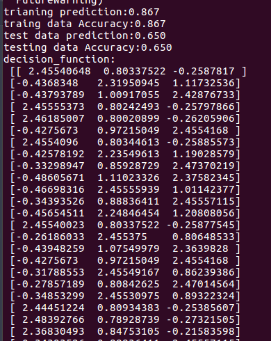
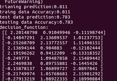
	print('trianing prediction:%.3f' %(clf.score(x_train, y_train)))
	# 预测值
	y_hat = clf.predict(x_train)
	show_accuracy(y_hat, y_train, 'traing data')
	print('test data prediction:%.3f' %(clf.score(x_test, y_test)))
	y_hat_test = clf.predict(x_test)
	show_accuracy(y_hat_test, y_test, 'testing data')

	# decision function
	print('decision_function:\n', clf.decision_function(x_train))
	# print('\npredict:\n', clf.predict(x_train).reshape(-1, 1))
	print('\npredict:\n', clf.predict(x_train))

	# 开始画图
	x1_min, x1_max = x[:, 0].min(), x[:, 0].max()
	x2_min, x2_max = x[:, 1].min(), x[:, 1].max()
	# 生成网格采样点
	x1, x2 = np.mgrid[x1_min:x1_max:200j, x2_min:x2_max:200j]
	# 测试点
	grid_test = np.stack((x1.flat, x2.flat), axis=1)
	print('grid_test:\n', grid_test)
	# 输出样本到决策面的距离
	z = clf.decision_function(grid_test)
	print('the distance to decision plane:\n', z)

	# 预测分类值
	grid_hat = clf.predict(grid_test)
	print('grid_hat:\n', grid_hat)
	# reshape grid_hat和x1形状一致
	grid_hat = grid_hat.reshape(x1.shape)

	cm_light = mpl.colors.ListedColormap(['#A0FFA0', '#FFA0A0', '#A0A0FF'])
	cm_dark = mpl.colors.ListedColormap(['g', 'b', 'r'])

	plt.pcolormesh(x1, x2, grid_hat, cmap=cm_light)
	# 样本点
	plt.scatter(x[:, 0], x[:, 1], c=np.squeeze(y), edgecolor='k', s=50, cmap=cm_dark)
	# 测试点
	plt.scatter(x_test[:, 0], x_test[:, 1], s=120, facecolor='none', zorder=10)
	plt.xlabel(iris_feature[0], fontsize=20)
	plt.ylabel(iris_feature[1], fontsize=20)
	plt.xlim(x1_min, x1_max)
	plt.ylim(x2_min, x2_max)
	plt.title('svm in iris data classification', fontsize=30)
	plt.grid()
	plt.show()

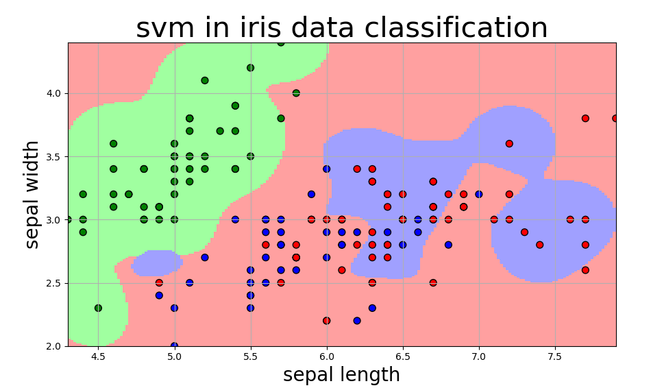
使用线性核函数：

输出中的decision function跟svm包中的svn函数参数decision_function_shape有关。ovo相当于把多分类问题分割为二分类问题求解，ovr相当于同时训练k个特征的分类器，然后把每个新的数据输入到分类器中，取得分最高的那个认定为属于该分类，有点像KNN思想。