So far, we have built a good understanding of how algorithmic trading works and how we can build trading signals from market data. We also looked into some basic trading strategies, as well as more sophisticated trading strategies, so it may seem like we are in a good place to start trading, right? Not quite. Another very important requirement
to be successful at algorithmic trading is understanding risk management and
using good risk management practices
.
Bad risk management practices
can
turn any good algorithmic trading strategy into
a
non profitable one
. On the other hand,
good risk management practices
can
turn a seemingly inferior [ɪnˈfɪriər]次的,较差的 trading strategy into
an
actually profitable one
. In this chapter, we will examine the different kinds of risk in algorithmic trading, look at how to quantitatively[ˈkwɑːntəteɪtɪvli] measure and compare these risks, and explore how to build a good risk management system to
adhere to循
these risk management practices.
In this chapter, we will cover the following topics:
- Differentiating between the types of risk and risk factors
- Quantifying the risk量化风险
- Differentiating between the measures of risk
- Making a risk management algorithm制定风险管理算法
Differentiating between the types of risk and risk factors
Risks
in algorithmic trading strategies can basically be of two things:
-
risks that
cause money loss
and -
risks that
cause illegal/forbidden behavior
in markets that cause regulatory actions[ˈreɡjələtɔːri]监管行动.
Let’s take a look at the risks involved before we look at what factors lead to increasing/decreasing these risks in the business of algorithmic trading.
Risk of trading losses
This is the most obvious and intuitive one—we want to trade to make money, but we always run through the risk of losing money against other market participants. Trading is a zero-sum game: some participants will make money, while some will lose money. The amount that’s lost by the losing participants is the amount that’s gained by the winning participants. This simple fact is what also makes trading quite challenging. Generally, less informed participants will lose money to more informed participants.
Informed
is a loose term here; it can mean participants with access to information that others don’t have. This can include
access to secretive or expensive or even illegal information sources, the ability to transport and consume such information that other participants don’t have
, and so on.
Information edge
信息优势 can also be gained by participants with a
superior ability to glean[ɡliːn]收集 information from the available information
, that is, some participants will have
better signals, better analytics abilities, and better predictive abilities
to edge out挤掉,淘汰 less informed participants. Obviously, more sophisticated participants will also beat less sophisticated participants.
Sophistication
can be gained from technology advantages as well, such as
faster reacting trading strategies
. The use of a low-level language such as C/C++ is harder to develop software in but allows us to build trading software systems that
react in single-digit microseconds processing time
.
-
An extreme speed advantage is available to participants that use
F
ield
P
rogrammable
G
ate
A
rray
s
(
FPGAs
)
to achieve sub-microsecond response times to market data updates. -
Another avenue of gaining sophistication is by
having more complex trading algorithms with more complex logic
that’s meant to squeeze out as much edge as possible.
It should be clear that algorithmic trading is an extremely complex and competitive business and that all the participants are doing their best to squeeze out every bit of profit possible by being
more informed and sophisticated
.
https://www.efinancialcareers.com/news/2017/07/xr-trading-2016
discusses an example of
trading losses
due to
decreased profitability
, which occurs due to
competition
among market participants
.
Regulation violation risks违规风险
The other risk that isn’t everyone’s first thought has to do with making sure that algorithmic trading strategies are not violating any regulatory rules. Failing to do so often results in astronomical[ˌæstrəˈnɑːmɪkl] fines天文罚款, massive legal fees巨额法律费用, and can often get participants banned from trading from certain or all exchanges. Since setting up successful algorithmic trading businesses are multi-year, multi-million dollar ventures[ˈventʃər]风险, getting shut down due to regulatory reasons can be crushing[ˈkrʌʃɪŋ]毁坏(某人的信心或幸福),令人沮丧. The SEC美国证券交易委员会(
https://www.sec.gov/
), FINRA美国金融业监管局(
https://www.finra.org/#/
), and CFTC美国商品期货交易委员会(
https://www.cftc.gov/
) are just some of many regulatory governing bodies watching over监视 algorithmic trading activity in equity股票, currency货币, futures期货, and options期权 markets.
These regulatory firms enforce执行 global and local regulations法规. In addition, the electronic trading exchanges themselves impose regulations and laws, the violation of which can also incur severe penalties. There are many market participants or algorithmic trading strategy behaviors that are forbidden. Some incur[ɪnˈkɜːr]招致,遭受 a warning or an audit and some incur penalties.
Insider trading reports
内幕交易报告 are quite well known by people inside and outside of the algorithmic trading business. While insider trading doesn’t really apply to algorithmic trading or high-frequency trading, we will introduce some of the common issues in algorithmic trading here.
This list is nowhere near complete, but these are
the top regulatory issues in algorithmic trading or high-frequency trading
.
Spoofing欺骗
Spoofing
[ˈspuːfɪŋ]电子欺骗 typically refers to the practice of
entering orders into the market that are not considered bonafide
[ˌboʊnə ˈfaɪdi]真正的,真实的. A
bonafide
order is one that
is entered with the intent of trading
. Spoofing orders are entered into the market
with the intent of misleading other market participants
, and these orders were
never entered with the intent of being executed
. The purpose of these orders is to make other participants believe that there are more real market participants who are willing to buy or sell than there actually are.
By spoofing on the bid
side通过在
喊价方(买入方,出价方,投标方)
进行
欺骗
,
-
market participants are
misled
into thinking there is
a lot of interest in buying
. -
This usually
leads to other market participants
adding more orders to
the bid side
and
moving or removing orders on
the ask side
卖出方 with
the expectation that prices will go up
. -
When prices go up, the spoofer then
sells
at a higher price
than would’ve been possible without the spoofing orders.
At this point, the
spoofer initiates
开始实施,发起
a
short
position and cancels all the spoofing bid orders
,
causing other market participants to do the same
. This
drive prices back down
from these synthetically raised higher prices. -
When prices have dropped sufficiently
, the spoofer then
buys at lower prices
to cover the short position and lock in a profit
.
Spoofing algorithms can repeat this over and over in markets that are mostly algorithmically trading and make a lot of money. This, however, is illegal in most markets because it
causes market price instability
, provides participants with misleading information about available market liquidity, and adversely affects负面影响 non-algorithmic trading investors/strategies. In summary, if such behavior was not made illegal, it would cause cascading instability连锁不稳定性 and make most market participants exit providing liquidity. Spoofing is treated as a serious violation in most electronic exchanges, and exchanges have sophisticated algorithms/monitoring systems to detect such behavior and flag标记 market participants who are spoofing.
The first case of spoofing got a lot of publicity, and those of you who are interested can learn more at
https://www.justice.gov/usao-ndil/pr/high-frequency-trader-sentenced-three-years-prison-disrupting-futures-market-first
Quote stuffing塞单或填鸭式报价行为
Quote stuffing is a manipulation tactic[ˈtæktɪk]策略,手法 that was employed被采用 by high-frequency trading participants. Nowadays, most exchanges have many rules that make quote stuffing infeasible[ɪnˈfizəbəl]不可实行的 as a profitable trading strategy. Quote stuffing is the practice行为 of
using very fast trading algorithms and hardware to enter, modify, and cancel large amounts of orders in one or more trading instruments
. Since each order action by a market participant causes the generation of public market data, it is possible for very fast participants to
generate a massive amount of market data and massively slow down slower participants who can no longer react in time
, thereby
causing profits for high-frequency trading algorithms
.
This is not as feasible in modern electronic trading markets, mainly because exchanges have
put in rules on messaging limits on individual market participants
. Exchanges have the ability to analyze and flag short-lived non-bonafide order flow标记短期的非真实订单流, and modern matching engines are able to better synchronize同步 market data feeds市场数据源 with order flow feeds订单流源.
https://www.businessinsider.com/huge-first-high-frequency-trading-firm-is-charged-with-quote-stuffing-and-manipulation-2010-9
discusses a recent quote stuffing market manipulation incident that caused regulatory actions.
Banging the close
冲击
收盘
Banging the close
is a disruptive[dɪsˈrʌptɪv]破坏的 and manipulative trading practice that still happens periodically[ˌpɪriˈɑːdɪkli]定期地,周期性地 in electronic trading markets, either intentionally or accidentally有意或无意地, by trading algorithms. This practice has to do with illegally manipulating the closing price of a derivative, also known as
the settlement price
最后结算价. Since
positions in
derivatives
markets such as
futures
期货 are marked at the settlement price at the end of the day
, this tactic[ˈtæktɪk]策略
uses large orders
during the final few minutes or seconds of closing where
many market participants are out of the market
already
to drive
less liquid market prices
in an illegal and disruptive way
.
This is, in some sense, similar to spoofing, but in this case, often, the participants banging the close may not pick up new executions during the closing period, but
may simply try to move market prices to make their already existing positions more profitable
. For cash- settled derivatives contracts,
the more favorable settlement price leads to more profit.
This is why trading closes are also monitored quite closely by
electronic trading derivative exchanges
to detect and flag this disruptive practice.
https://www.cftc.gov/PressRoom/PressReleases/5815-10
discusses an incident of banging the close for those who are interested.
Sources of risk风险来源
Now that we have a good understanding of the different kinds of risk in algorithmic trading, let’s look at
the factors
in
algorithmic trading strategy development, optimization, maintenance, and operation
that
causes
them
.
Software implementation risk
A modern algorithmic trading business is essentially a technology business, hence giving birth to the new term
FinTech
to mean the intersection of
fin
ance
and
tech
nology
. Computer software is designed, developed, and tested by
humans who are error-prone
and sometimes, these errors creep[kriːp]蔓延 into trading systems and algorithmic trading strategies.
Software implementation bugs are often the most overlooked被忽视的 source of risk in algorithmic trading
. While operation risk and market risk are extremely important, software implementation bugs have the potential to cause millions of dollars in losses, and there have been many cases of firms going bankrupt due to software implementation bugs within minutes.
In recent times, there was the infamous Knight Capital incident, where a software implementation bug combined with an operations risk issue caused them to lose $440 million within 45 minutes and they ended up getting shut down. Software implementation bugs are also very tricky棘手 because software engineering is a very complex process, and when we add the additional complexity of having sophisticated and complex algorithmic trading strategies and logic, it is hard to guarantee that the implementation of trading strategies and systems are safe from bugs. More information can be found at
https://dealbook.nytimes.com/2012/08/02/knight-capital-says-trading-mishap-cost-it-440-million/
.
Modern algorithmic trading firms have rigorous[ˈrɪɡərəs](规则,制度等)严格的,苛刻的 software development practices to safeguard themselves against software bugs. These include
-
rigorous unit tests
, which
are small tests on individual software components
to verify their behavior doesn’t change to an incorrect behavior as
software development/maintenance being made to existing components
is performed
. -
There are also
regression tests
, which are tests that
test larger components
that are composed of smaller components
as a whole
to ensure the higher-level behavior remains consistent
. -
All electronic trading exchanges also provide
a test market environment
with test market data feeds
and
test order entry interfaces
where market participants have to build, test, and certify[ˈsɜːrtɪfaɪ]验证 their components with the exchange before they are even allowed to trade in live markets.
Most sophisticated algorithmic trading participants also have
backtesting
software that simulates a trading strategy over historically recorded data to ensure strategy behavior is in line with expectations. We will explore
backtesting
further in Chapter 9 , Creating a
Backtester
in Python. Finally, other software management practices, such as
code reviews and change management,
are also performed on a daily basis to verify the integrity完整性 of algorithmic trading systems and strategies on a daily basis. Despite all of these precautions[prɪˈkɔːʃn]预防措施, software implementation bugs do slip into live trading markets, so we should always be aware警惕 and cautious谨慎 because software is never perfect and the cost of mistakes/bugs is very high in the algorithmic trading business, and even higher in the HFT(High-frequency trading) business.
DevOps risk开发运营风险
DevOps risk
is the term that is used to describe
the risk potential when
algorithmic trading strategies are deployed to live markets
. This involves building and deploying correct trading strategies and configuring the configuration, the signal parameters, the trading parameters, and starting, stopping, and monitoring them. Most modern trading firms trade markets electronically almost 23 hours a day, and they have
a large number of staff whose only job is to keep an eye on the automated algorithmic trading strategies
that are deployed to live markets to ensure they are behaving as expected and
no erroneous
[ɪˈroʊniəs]
没有错误的
behavior goes uninvestigated不予调查. They are known as the Trading Desk, or TradeOps or DevOps.
These
people
have a decent understanding有足够理解 of software development, trading rules, and exchange for provided risk monitoring interfaces. Often, when software implementation bugs end up going to live markets, they
are the final line of defense
最后一道防线
, and it is
their job to
monitor the systems, detect issues, safely pause or stop the algorithms, and contact and resolve the issues that have emerged
. This is the most common understanding of where
operation risk
can show up. Another source of operation risk is in algorithmic trading strategies that are not 100% black box.
Black box trading strategies
are trading strategies that
do not require any human feedback or interaction
. These are started at a certain time and then stopped at a certain time, and
the algorithms themselves make all the decisions
.
Gray box trading strategies
are trading strategies that are not 100% autonomous. These strategies still have
a lot of automated decision-making built into them
, but they also have
external controls
that
allow
the traders or TradeOps engineers
to monitor the strategies
, as well as
adjust parameters and trading strategy behavior, and even send manual orders
. Now, during these
manual human interventions
, there is another source of risk, which is basically
the risk of humans making mistakes
in the commands/adjustments
that are sent to these strategies.
Sending incorrect parameters can cause the algorithm to behave incorrectly and cause losses.
There are also cases of sending bad commands, which can cause an unexpected and unintentional large impact on the market, causing trading losses and market disruptions市场混乱 that add regulatory fines. One of the common errors is the
fat finger error,
where prices, sizes, and buy/sell instructions are sent incorrectly due to a fat finger. Some examples can be found at
https://www.bloomberg.com/news/articles/2019-01-24/oops-a-brief-history-of-some-of-the-market-s-worst-fat-fingers
Market risk
Finally, we have market risk, which is what is commonly thought of when we think of risk in algorithmic trading. This is the risk of
trading against
and
losing money to
more informed participants
. Every market participant, at some point or the other, on some trade or the other, will lose money to a more informed participant. We discussed what makes an informed participant superior to a non-informed one in the previous section. Obviously,
the only way to
avoid market risk
is to get access to more information, improve the trading edge, improve sophistication, and improve technology advantages
. But since market risk is a truth of all algorithmic trading strategies, a very important aspect is to
understand the behavior of the algorithmic trading strategy
before deploying it to live markets.
This involves understanding what to expect normal behavior to look like and, more importantly, understanding when a certain strategy makes and loses money and
quantifying loss metrics to set up expectations
. Then,
risk limits
are set up at multiple places in an algorithmic trading pipeline in the trading strategy, then in a central risk monitoring system, then in the order gateway, sometimes at the clearing firm, and finally sometimes even at the exchange level. Each
extra layer of risk check
can slow down a market participant’s ability to react to fast-moving markets, but it is essential to have these to prevent runaway失控的 trading algorithms from causing a lot of damage.
Once
the trading strategy has violated maximum trading risk limits assigned to
it, it will be shut down at one or more places where the risk validation is set up.
Market risk
is very important to understand, implement, and configure correctly because
incorrect risk estimates can kill a profitable trading strategy
by increasing the frequency and magnitude of losing trades, losing positions, losing days, and even losing weeks or months. This is because the trading strategy could have
lost its profitable edge
盈利优势 and if you leave it running for too long
without adapting it to changing markets
, it can erode[ɪˈroʊd] 侵蚀,腐蚀,削弱,降低 all the profits the strategy may have generated in the past. Sometimes, m
arket conditions are very different than what is expected and strategies can go through periods of larger than normal losses
, in which cases it is important to have risk limits set up to detect outsized losses and adjust trading parameters or stop trading.
We will look at研究 what risk measures are common in algorithmic trading, how to quantify and research them from historical data, and how to configure and calibrate algorithmic strategies before deploying them to live markets. For now, the summary is that market risk is a normal part of algorithmic trading, but failing to understand and prepare for it can destroy a lot of good trading strategies.
Quantifying the risk量化风险
Now, let’s get started with understanding what realistic risk constraints look like and how to quantify them. We will list, define, and implement some of the most commonly used risk limits in the modern algorithmic trading industry today. We will use the
volatility adjusted mean reversion strategy
we built in
https://blog.csdn.net/Linli522362242/article/details/121896073
, Sophisticated Algorithmic Strategies, as our realistic trading strategy, which we now need to
define and quantify risk measures for
.
The severity of risk violations风险违规的严重程度
One thing to understand before diving into all the different risk measures is defining what the severity[sɪˈverəti] of a risk violation means. So far, we’ve been discussing risk violations as being maximum risk limit violations. But in practice, there are multiple levels of every risk limit, and each level of risk limit violation is not equally as catastrophic[ˌkætəˈstrɑːfɪk]灾难性的 to algorithmic trading strategies.
The lowest severity risk violation
would be considered
a warning risk violation
, which means that this risk violation, while not expected to happen regularly定期发生, can happen normally during a trading strategy operation. Intuitively, it is easy to think of this as, say, on most days, trading strategies do not send more than 5,000 orders a day, but on certain
volatile days
, it is possible and acceptable that the trading strategy sends 20,000 orders on that day. This would be considered an example of a warning risk violation – this is unlikely, but not a sign of trouble. The purpose of this risk violation is
to warn the trader that something unlikely is happening in the market or trading strategy
.
The next level of risk violation
is what would be considered as something where
the strategy is still functioning correctly正常运行 but has reached the limits of what it is allowed to do, and must safely liquidate[ˈlɪkwɪdeɪt]清算,清理债务 and shut down
. Here, the strategy is allowed to
send orders and make trades that flatten the position and cancel new entry orders
, if there are any. Basically,
the strategy is done trading but is allowed to automatically handle the violation and finish trading until a trader checks on what happens and decides to either restart and allocate higher risk limits to the trading strategy
.
The final level of risk violation
is what would be considered
a maximum possible risk violation
, which is a violation that
should never, ever happen
. If a trading strategy ever triggers this risk violation, it is a sign that something went very wrong. This risk violation means that
the strategy is no longer allowed to send any more order flow to the live markets
. This risk violation would
only be triggered during periods of extremely unexpected events
, such as a flash crash market condition闪电崩盘市场条件. This severity of risk violation basically means that the algorithmic trading strategy is not designed to deal with such an event automatically and must
freeze trading and then resort to external operators to manage
open positions未结头寸
and live orders
.
Differentiating the measures of risk
Let’s explore different measures of risk. We will use the trading performance from
the volatility adjusted mean reversion strategy
we saw in
https://blog.csdn.net/Linli522362242/article/details/121896073
, Sophisticated Algorithmic Strategies, as an example of a trading strategy in which we wish to
understand the risks behind and quantify and calibrate them
.
In t5
https://blog.csdn.net/Linli522362242/article/details/121896073
, Sophisticated Algorithmic Trading Strategies, we built the Mean Reversion,
Volatility Adjusted Mean Reversion
, Trend Following, and
Volatility Adjusted Trend Following strategies
. These can be found in
https://blog.csdn.net/Linli522362242/article/details/121896073
, Sophisticated Algorithmic Strategies, in the
Mean reversion strategy(+APO+
StdDev
) that
dynamically adjusts
for changing volatility
section. Let’s load up the trading performance . csv file, as shown in the following code block, and quickly look at what fields we have available:
import pandas as pd
import pandas_datareader.data as pdr

def load_financial_data( start_date, end_date, output_file='', stock_symbol='GOOG' ):
    if len(output_file) == 0:
        output_file = stock_symbol+'_data_large.pkl'

    try:
        df = pd.read_pickle( output_file )
        print( "File {} data found...reading {} data".format( output_file ,stock_symbol) )
    except FileNotFoundError:
        print( "File {} not found...downloading the {} data".format( output_file, stock_symbol ) )
        df = pdr.DataReader( stock_symbol, "yahoo", start_date, end_date )
        df.to_pickle( output_file )
    return df

goog_data = load_financial_data( stock_symbol='GOOG',
                                 start_date='2014-01-01',
                                 end_date='2018-01-01',
                                 output_file='goog_data.pkl'
                               )
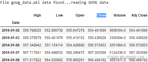
goog_data.head()
# Variables/constants for EMA Calculation:
NUM_PERIODS_FAST_10 = 10 # Static time period parameter for the fast EMA
K_FAST = 2/(NUM_PERIODS_FAST_10 + 1) # Static smoothing factor parameter for fast EMA
ema_fast = 0 # initial ema
ema_fast_values = [] # we will hold fast EMA values for visualization purpose

NUM_PERIODS_SLOW_40 = 40 # Static time period parameter for the slow EMA
K_SLOW = 2/(NUM_PERIODS_SLOW_40 + 1) # Static smoothing factor parameter for slow EMA
ema_slow = 0 # initial ema
ema_slow_values = [] # we will hold slow EMA values for visualization purpose

apo_values = [] # track computed absolute price oscillator values

# Variables for Trading Strategy trade, position & pnl management:

# Container for tracking buy/sell order,
# +1 for buy order, -1 for sell order, 0 for no-action
orders = []

# Container for tracking positions,
# positive for long positions, negative for short positions, 0 for flat/no position
positions = []

# Container for tracking total_pnls, this is the sum of
# closed_pnl i.e. pnls already locked in
# and open_pnl i.e. pnls for open-position marked to market price
pnls = []


last_buy_price = 0  # used to prevent over-trading at/around the same price
last_sell_price = 0 # used to prevent over-trading at/around the same price
position = 0 # Current position of the trading strategy

# Summation of products of
# buy_trade_price and buy_trade_qty for every buy Trade made
# since last time being flat
buy_sum_price_qty = 0
# Summation of buy_trade_qty for every buy Trade made since last time being flat
buy_sum_qty = 0

# Summation of products of
# sell_trade_price and sell_trade_qty for every sell Trade made
# since last time being flat
sell_sum_price_qty = 0
# Summation of sell_trade_qty for every sell Trade made since last time being flat
sell_sum_qty = 0

open_pnl = 0   # Open/Unrealized PnL marked to market
closed_pnl = 0 # Closed/Realized PnL so far

# Constants that define strategy behavior/thresholds

# APO trading signal value below which(-10) to enter buy-orders/long-position
APO_VALUE_FOR_BUY_ENTRY = -10 # (oversold, expect a bounce back up)
# APO trading signal value above which to enter sell-orders/short-position
APO_VALUE_FOR_SELL_ENTRY = 10 # (overbought, expect a bounce back down)

# Minimum price change since last trade before considering trading again,
MIN_PRICE_MOVE_FROM_LAST_TRADE = 10 # this is to prevent over-trading at/around same prices
NUM_SHARES_PER_TRADE = 10

# positions are closed if currently open positions are profitable above a certain amount,
# regardless of APO values.
# This is used to algorithmically lock profits and initiate more positions
# instead of relying only on the trading signal value.

# Minimum Open/Unrealized profit at which to close positions and lock profits
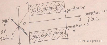
MIN_PROFIT_TO_CLOSE = 10*NUM_SHARES_PER_TRADE
import statistics as stats
import math as math

data2 = goog_data.copy()
close = data2['Close']

# Constants/variables that are used to compute standard deviation as a volatility measure
SMA_NUM_PERIODS_20 = 20 # look back period
price_history = []      # history of prices

for close_price in close:
    price_history.append( close_price )
    if len( price_history) > SMA_NUM_PERIODS_20 : # we track at most 'time_period' number of prices
        del ( price_history[0] )

    # calculate vairance during the SMA_NUM_PERIODS_20 periods
    sma = stats.mean( price_history )
    variance = 0 # variance is square of standard deviation
    for hist_price in price_history:
        variance = variance + ( (hist_price-sma)**2 )

    stddev = math.sqrt( variance/len(price_history) )

    # a volatility factor that ranges from 0 to 1
    stddev_factor = stddev/15 # 15 since since the population stddev.mean() = 15.45
    # closer to 0 indicate very low volatility,
    # around 1 indicate normal volatility
    # > 1 indicate above-normal volatility
    if stddev_factor == 0:
        stddev_factor = 1

    # This section updates fast and slow EMA and computes APO trading signal
    if (ema_fast==0): # first observation
        ema_fast = close_price # initial ema_fast or ema_slow
        ema_slow = close_price
    else:
        # ema fomula
        # K_FAST*stddev_factor or K_SLOW*stddev_factor
        # more reactive to newest observations during periods of higher than normal volatility
        ema_fast = (close_price-ema_fast) * K_FAST*stddev_factor + ema_fast
        ema_slow = (close_price-ema_slow) * K_SLOW*stddev_factor + ema_slow

    ema_fast_values.append( ema_fast )
    ema_slow_values.append( ema_slow )

    apo = ema_fast - ema_slow
    apo_values.append( apo )

    # 6. This section checks trading signal against trading parameters/thresholds and positions, to trade.

    # We will perform a sell trade at close_price if the following conditions are met:
    # 1. The APO trading signal value(positive) > Sell-Entry threshold (overbought, expect a bounce back down, sell for profit)
    #     and the difference between current-price and last trade-price is different enough.(>Minimum price change)
    # 2. We are long( +ve position ) and
    #    either APO trading signal value >= 0 or current position is profitable enough to lock profit.
    # APO_VALUE_FOR_SELL_ENTRY * stdev_factor:
    #              by increasing the threshold for entry by a factor of volatility,
    #              makes us less aggressive in entering positions(here is sell) during periods of higher volatility,
    # dynamic MIN_PROFIT_TO_CLOSE / stddev_factor:
    #              to decrease the the expected profit threshold during periods of increased volatility
    #              to be more aggressive in exciting positions
    #              it is riskier to hold on to positions for longer periods of time.
    if ( ( apo > APO_VALUE_FOR_SELL_ENTRY*stddev_factor and \
           abs( close_price-last_sell_price ) > MIN_PRICE_MOVE_FROM_LAST_TRADE*stddev_factor
         )
         or
         ( position>0 and (apo >=0 or open_pnl > MIN_PROFIT_TO_CLOSE/stddev_factor ) )
       ): # long from -ve APO and APO has gone positive or position is profitable, sell to close position
        orders.append(-1) # mark the sell trade
        last_sell_price = close_price
        position -= NUM_SHARES_PER_TRADE
        sell_sum_qty += NUM_SHARES_PER_TRADE
        sell_sum_price_qty += (close_price * NUM_SHARES_PER_TRADE) # update vwap sell-price
        print( "Sell ", NUM_SHARES_PER_TRADE, " @ ", close_price, "Position: ", position )

    # 7. We will perform a buy trade at close_price if the following conditions are met:
    # 1. The APO trading signal value(negative) < below Buy-Entry threshold (oversold, expect a bounce back up, buy for future profit)
    #    and the difference between current-price and last trade-price is different enough.(>Minimum price change)
    # 2. We are short( -ve position ) and
    #    either APO trading signal value is <= 0 or current position is profitable enough to lock profit.
    # APO_VALUE_FOR_BUY_ENTRY * stdev_factor:
    #              by increasing the threshold for entry by a factor of volatility,
    #              makes us less aggressive in entering positions(here is sell) during periods of higher volatility,
    # dynamic MIN_PROFIT_TO_CLOSE / stddev_factor:
    #              to decrease the the expected profit threshold during periods of increased volatility
    #              to be more aggressive in exciting positions
    #              it is riskier to hold on to positions for longer periods of time.
    elif ( ( apo < APO_VALUE_FOR_BUY_ENTRY*stddev_factor and \
             abs( close_price-last_buy_price ) > MIN_PRICE_MOVE_FROM_LAST_TRADE*stddev_factor
           )
           or
           ( position<0 and (apo <=0 or open_pnl > MIN_PROFIT_TO_CLOSE/stddev_factor ) )
         ): # short from +ve APO and APO has gone negative or position is profitable, buy to close position
        orders.append(+1) # mark the buy trade
        last_buy_price = close_price
        position += NUM_SHARES_PER_TRADE
        buy_sum_qty += NUM_SHARES_PER_TRADE
        buy_sum_price_qty += (close_price * NUM_SHARES_PER_TRADE) # update the vwap buy-price
        print( "Buy ", NUM_SHARES_PER_TRADE, " @ ", close_price, "Position: ", position )
    else:
        # No trade since none of the conditions were met to buy or sell
        orders.append( 0 )

    positions.append( position )

    # 8. The code of the trading strategy contains logic for position/PnL management.
    #    It needs to update positions and compute open and closed PnLs when market prices change
    #    and/or trades are made causing a change in positions

    # This section updates Open/Unrealized & Closed/Realized positions
    open_pnl = 0
    if position > 0:
        # long position and some sell trades have been made against it,
        # close that amount based on how much was sold against this long position
        # PnL_realized = sell_sum_qty * (Average Sell Price - Average Buy Price)
        if sell_sum_qty > 0:           # vwap for sell                   # vwap  for buy
            open_pnl = sell_sum_qty * (sell_sum_price_qty/sell_sum_qty - buy_sum_price_qty/buy_sum_qty)
        # mark the remaining position to market
        # i.e. pnl would be what it would be if we closed at current price
        # sell
        # position -= NUM_SHARES_PER_TRADE
        # sell_sum_qty += NUM_SHARES_PER_TRADE
        # PnL_unrealized = remaining position * (Exit Price - Average Buy Price)
        # if now, sell sell_sum_qty @ any price, we should use abs(position-sell_sum_qty) *
        open_pnl += abs(position) * ( close_price - buy_sum_price_qty/buy_sum_qty )
        # print( position, (buy_sum_qty-sell_sum_qty), open_pnl)
    elif position < 0:
        # short position and some buy trades have been made against it,
        # close that amount based on how much was bought against this short position
        # PnL_realized = buy_sum_qty * (Average Sell Price - Average Buy Price)
        if buy_sum_qty > 0:           # vwap for sell                   # vwap  for buy
            open_pnl = buy_sum_qty * (sell_sum_price_qty/sell_sum_qty - buy_sum_price_qty/buy_sum_qty)
        # mark the remaining position to market
        # i.e. pnl would be what it would be if we closed at current price
        # buy
        # position += NUM_SHARE_PER_TRADE
        # buy_sum_qty += NUM_SHARE_PER_TRADE
        # PnL_unrealized = remaining position * (Average Sell Price - Exit Price)
        # if now, buy buy_sum_qty @ any price, we should use abs(position-buy_sum_qty) *
        open_pnl += abs(position) * ( sell_sum_price_qty/sell_sum_qty - close_price )
        # print( position, (buy_sum_qty-sell_sum_qty), open_pnl)
    else:
        # flat, so update closed_pnl and reset tracking variables for positions & pnls
        closed_pnl += (sell_sum_price_qty - buy_sum_price_qty)

        buy_sum_price_qty = 0
        buy_sum_qty = 0
        last_buy_price = 0

        sell_sum_price_qty = 0
        sell_sum_qty = 0
        last_sell_price = 0

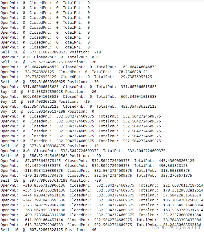
    print( "OpenPnL: ", open_pnl, " ClosedPnL: ", closed_pnl, " TotalPnL: ", (open_pnl + closed_pnl) )
    pnls.append(closed_pnl + open_pnl)
# This section prepares the dataframe from the trading strategy results and visualizes the results
data2 = data2.assign( ClosePrice = pd.Series(close, index=data2.index) )
data2 = data2.assign( Fast10DayEMA = pd.Series(ema_fast_values, index=data2.index) )
data2 = data2.assign( Slow40DayEMA = pd.Series(ema_slow_values, index=data2.index) )
data2 = data2.assign( APO = pd.Series(apo_values, index=data2.index) )
data2 = data2.assign( Trades = pd.Series(orders, index=data2.index) )
data2 = data2.assign( Position = pd.Series(positions, index=data2.index) )
data2 = data2.assign( Pnl = pd.Series(pnls, index=data2.index) )
import matplotlib.pyplot as plt
fig = plt.figure( figsize=(20,10) )
data2['ClosePrice'].plot(color='k', lw=3., legend=True)
data2['Fast10DayEMA'].plot(color='y', lw=1., legend=True)
data2['Slow40DayEMA'].plot(color='m', lw=1., legend=True)
plt.plot( data2.loc[ data2.Trades == 1 ].index, data2.ClosePrice[data2.Trades == 1 ],
color='y', lw=0, marker='^', markersize=7, label='buy'
)
plt.plot( data2.loc[ data2.Trades == -1 ].index, data2.ClosePrice[data2.Trades == -1 ],
color='b', lw=0, marker='v', markersize=7, label='sell'
)
plt.autoscale(enable=True, axis='x', tight=True)
plt.legend()
plt.show()
more aggressive in exiting positions
during periods of increased volatility
(for example,

VS

), because as we discussed before, during
periods of higher than normal volatility
, it is
riskier to hold on to positions for longer periods of time
.
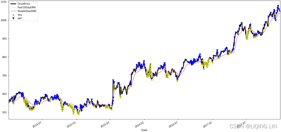
fig = plt.figure( figsize=(20,10) )

data2['APO'].plot(color='k', lw=3., legend=True)
plt.plot( data2.loc[ data2.Trades == 1 ].index, data2.APO[data2.Trades == 1 ],
          color='y', lw=0, marker='^', markersize=7, label='buy'
        )
plt.plot( data2.loc[ data2.Trades == -1 ].index, data2.APO[data2.Trades == -1 ],
          color='b', lw=0, marker='v', markersize=7, label='sell'
        )
plt.axhline(y=0, lw=0.5, color='k')
for i in range( APO_VALUE_FOR_BUY_ENTRY, APO_VALUE_FOR_BUY_ENTRY*5, APO_VALUE_FOR_BUY_ENTRY ):
  plt.axhline(y=i, lw=0.5, color='r')
for i in range( APO_VALUE_FOR_SELL_ENTRY, APO_VALUE_FOR_SELL_ENTRY*5, APO_VALUE_FOR_SELL_ENTRY ):
  plt.axhline(y=i, lw=0.5, color='g')

plt.autoscale(enable=True, axis='x', tight=True)
plt.legend()

plt.show()
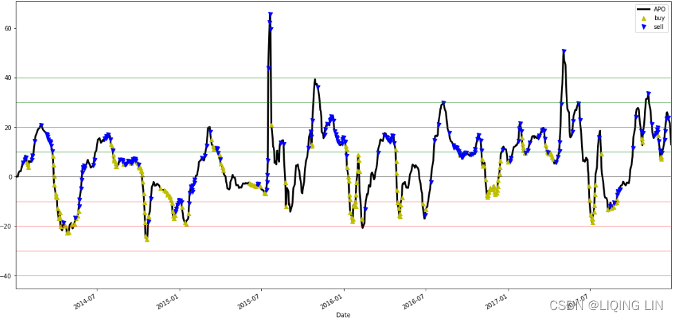
fig = plt.figure( figsize=(20,10))

data2['Position'].plot(color='k', lw=1., legend=True)
plt.plot( data2.loc[ data2.Position == 0 ].index, data2.Position[ data2.Position == 0 ],
          color='r', lw=0, marker='.', label='flat'
        )
plt.plot( data2.loc[ data2.Position > 0 ].index, data2.Position[ data2.Position > 0 ],
          color='y', lw=0, marker='+', label='long'
        )
plt.plot( data2.loc[ data2.Position < 0 ].index, data2.Position[ data2.Position < 0 ],
          color='b', lw=0, marker='_', label='short'
        )
plt.axhline(y=0, lw=0.5, color='k')
for i in range( NUM_SHARES_PER_TRADE, NUM_SHARES_PER_TRADE*25, NUM_SHARES_PER_TRADE*5 ):
  plt.axhline(y=i, lw=0.5, color='r')
for i in range( -NUM_SHARES_PER_TRADE, -NUM_SHARES_PER_TRADE*25, -NUM_SHARES_PER_TRADE*5 ):
  plt.axhline(y=i, lw=0.5, color='g')

plt.autoscale(enable=True, axis='x', tight=True)
plt.legend()
plt.show()
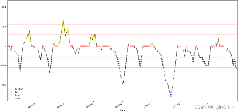
fig = plt.figure( figsize=(20,10))

plt.plot( data.index, data['Pnl'], color='g', lw=1.,
          label='BasicMeanReversionPnL'
        )#########################
plt.plot( data.loc[ data.Pnl > 0 ].index, data.Pnl[ data.Pnl > 0 ],
          color='y', lw=0, marker='.',
          #label='Pnl'
        )
plt.plot( data.loc[ data.Pnl < 0 ].index, data.Pnl[ data.Pnl < 0 ],
          color='r', lw=0, marker='.',
          #label='Pnl'
        )

plt.plot( data2.index, data2['Pnl'], color='b', lw=1.,
          label='VolatilityAdjustedMeanReversionPnL'
        )#########################
plt.plot( data2.loc[ data.Pnl > 0 ].index, data2.Pnl[ data.Pnl > 0 ],
          color='y', lw=0, marker='.',
          #label='Pnl'
        )
plt.plot( data2.loc[ data.Pnl < 0 ].index, data2.Pnl[ data.Pnl < 0 ],
          color='r', lw=0, marker='.',
          #label='Pnl'
        )
plt.axhline(y=15000, ls='--', alpha=0.5)
plt.autoscale(enable=True, axis='x', tight=True)
plt.legend()
plt.show()
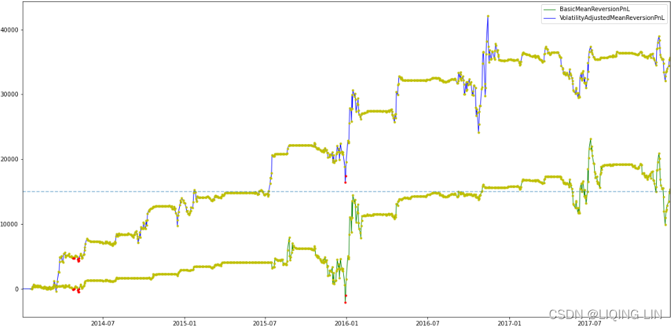
In this case, dynamically adjusts(StdDev(
![]()
and
![]()
) plus APO) the trading strategy(here is the Mean Reversion Strategy) for volatility increases the strategy(Mean Reversion Strategy) performance by 200%!
data2.head(n=5)

data2.to_csv("volatility_adjusted_mean_reversion_apo_stddev.csv", sep=",")Let’s load up the trading performance . csv file, as shown in the following code block, and quickly look at what fields we have available:
import pandas as pd
import matplotlib.pyplot as plt

results = pd.read_csv('volatility_adjusted_mean_reversion_apo_stddev.csv')
print( results.head(1) )

For the purposes of implementing and quantifying risk measures
, the fields we are interested in are
Date, High, Low, ClosePrice, Trades, Position, and PnL
. We will ignore the other fields since we do not require them for the risk measures we are currently interested in. Now, let’s dive into understanding and implementing our risk measures.
Stop-loss(PnL is the cumulative result)
The first risk limit we will look at is quite intuitive and is called
stop-loss
, or
max-loss
. This
limit is the maximum amount of money a strategy is allowed to lose
, that is, the
minimum PnL allowed
. This often has a notion of a time frame for that loss, meaning
stop-loss can be for a day, for a week, for a month, or for the entire lifetime of the strategy
. A stop-loss with a time frame of a day means that if the strategy loses a stop-loss amount of money in a single day,
it is not allowed to trade any more on that day, but can resume the next day
. Similarly, for a stop-loss amount in a week, it is not allowed to trade anymore for that week, but can resume next week.
Now, let’s
compute stop-loss levels on a week and month
for the volatility adjusted mean reversion strategy, as shown in the following code:
num_days = len( results.index ) # results.index : RangeIndex(start=0, stop=1007, step=1)

pnl = results['Pnl']

weekly_losses = []
monthly_losses = []

for i in range( 0, num_days ):
    if i>=5 and pnl[i-5] > pnl[i]:
        weekly_losses.append( pnl[i] - pnl[i-5] )

    if i>=20 and pnl[i-20] > pnl[i]:
        monthly_losses.append( pnl[i] - pnl[i-20] )

figure = plt.figure(figsize=(10,6))
plt.hist( weekly_losses, 50 )
plt.gca().set( title='Weekly Loss Distribution',
               xlabel='pnl $', ylabel='Frequency'
             )
plt.show()
Let’s have a look at the
weekly loss distribution
plot shown here :
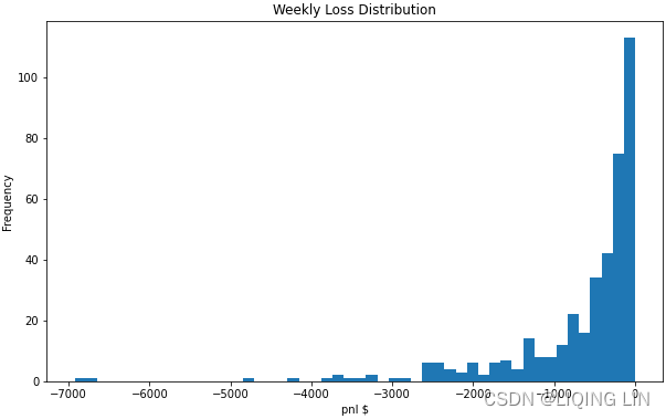
figure = plt.figure(figsize=(10,6))
plt.hist( monthly_losses, 50 )
plt.gca().set( title='Monthly Loss Distribution',
               xlabel='pnl $', ylabel='Frequency'
             )
plt.show()
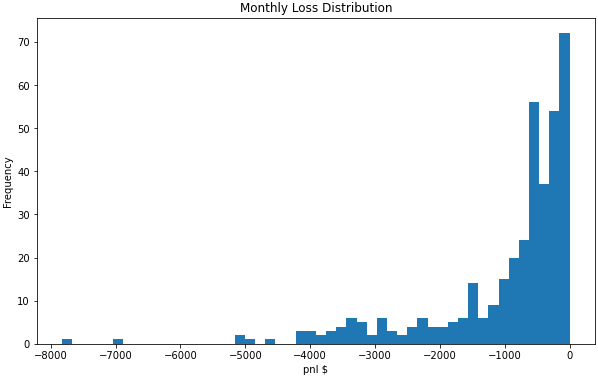
The plots show the distribution of weekly and monthly losses. From these, we can observe the following:
-
A weekly loss
of anything more than $3K and
a monthly loss
of anything more than $4K is highly unexpected. - A weekly loss of more than $7K and a monthly loss of $8K have never happened, so it can be considered an unprecedented[ʌnˈpresɪdentɪd]前所未有的,史无前例的 event, but we will revisit this later.
Max drawdown最大回撤
Max drawdown is also a PnL metric, but this
measures the maximum loss that a strategy can take over a series of days衡量的是策略在一系列天数内可以承受的最大损失
. This is defined as the
peak to trough
[trɔːf]波谷 decline in a
trading strategy’s account value
. This is important as a risk measure so that we can get an idea of what
the historical maximum decline历史最大跌幅
in the account value can be. This is important because we can get unlucky during the deployment of a trading strategy and run it in live markets right at the beginning of the drawdown.
Having an expectation of what the maximum drawdown is can help us understand whether the strategy loss streak连续亏损 is still within our expectations or whether something unprecedented is happening. Let’s look at how to compute it:
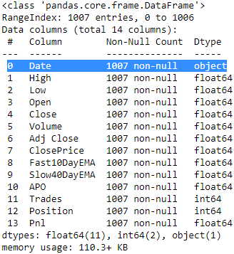
results.info()
results['Date']=pd.to_datetime( results['Date'] ) # convert Dtype in the 'Date' column to datetime
results=results.set_index(['Date'])  # set the 'Date' column as index
results.head()

max_pnl = 0
max_drawdown = 0
drawdown_max_pnl = 0
drawdown_min_pnl = 0

for i in range(0, num_days):
    max_pnl = max( max_pnl, pnl[i] )
    drawdown = max_pnl - pnl[i] # get the decline

    if drawdown > max_drawdown:
        max_drawdown = drawdown # maximum decline
        drawdown_max_pnl = max_pnl # peak
        drawdown_min_pnl = pnl[i]  # trough

print( 'Max Drawdown:', max_drawdown )
print( 'Max PnL', drawdown_max_pnl)
print( 'Min PnL', drawdown_min_pnl)

figure = plt.figure( figsize=(10,6) )
results['Pnl'].plot( x='Date' )
plt.axhline( y=drawdown_max_pnl, color='g' )
plt.axhline( y=drawdown_min_pnl, color='r' )
plt.gca().set( xlabel='Date', ylabel='Pnl' )

plt.show()
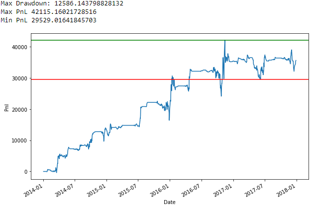
In the plot, the max drawdown occurs roughly during the period of 2016-07-01 to 2017-07-01 of this PnL series, with the
maximum PnL
being 42K and the
minimum PnL
after that high being 29K, causing the maximum drawdown achieved to be roughly 12K:
max_pnl = 0
max_drawdown = 0
drawdown_max_pnl = 0
drawdown_min_pnl = 0

for i in range(0, num_days):
    max_pnl = max( max_pnl, pnl[i] )
    drawdown = max_pnl - pnl[i] # get the decline

    if drawdown > max_drawdown:
        max_drawdown = drawdown # maximum decline
        drawdown_max_pnl = max_pnl # peak
        drawdown_min_pnl = pnl[i]  # trough

print( 'Max Drawdown:', max_drawdown )
print( 'Max PnL', drawdown_max_pnl)
print( 'Min PnL', drawdown_min_pnl)

figure = plt.figure( figsize=(10,6) )
# .loc['2016-07-01':'2017-07-01']
results.loc['2016-07-01':'2017-07-01']['Pnl'].plot( x='Date' )
plt.axhline( y=drawdown_max_pnl, color='g' )
plt.axhline( y=drawdown_min_pnl, color='r' )
plt.gca().set( xlabel='Date', ylabel='Pnl' )

plt.show()
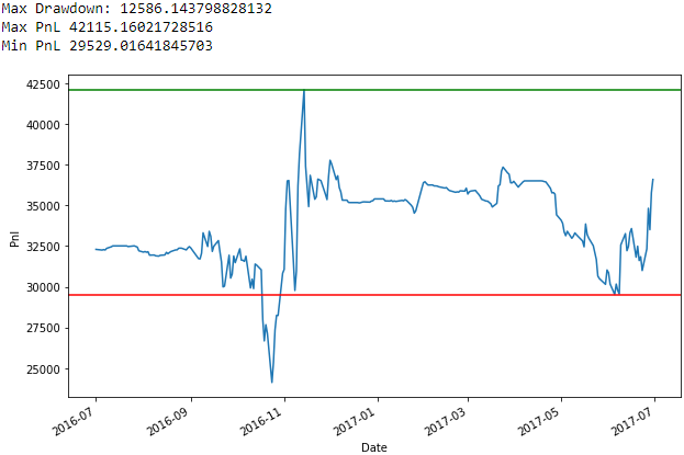
The plot is simply the same plot as before but zoomed in to the exact observations where the drawdown occurs. As we mentioned previously, after achieving a high of roughly 42K, PnLs have a large drawdown of 12K and drop down to roughly 29K, before rebounding.
Position limits( from
d
istribution of the positions
)
Position limits
are also quite straightforward and intuitive to understand. It is simply the maximum position, long or short, that the strategy should have at any point in its trading lifetime. It is possible to have
two different position limits, one for the
maximum long position
and another for
the maximum short position
, which can be useful, for instance, where
shorting stocks
have
different rules/risks
associated with
them
than being
long on stocks does
. Every unit of open position has a risk associated with it. Generally,
the larger the position
a strategy puts on,
the larger the risk
associated with it. So,
the best strategies
are the ones that can
make money
while getting into
as small a position as possible
. In either case, before a strategy is deployed to production, it is important
to
quantify and estimate what the maximum positions the strategy can get into, based on historical performance
, so that we can
find out
when a strategy is
within its normal behavior parameters
and when it is
outside of historical norms
.
Finding the maximum position
is straightforward. Let’s find a quick
distribution of the positions
with the help of the following code:
position = results['Position']

figure = plt.figure( figsize=(10,6) )
plt.rcParams.update({'font.size': 12})

plt.hist( position, bins=20 ) # If bins is an integer, it defines the number of equal-width bins in the range.
plt.gca().set( title='Position Distribution',
               xlabel='Shares', ylabel='Frequency',
             )
plt.show()
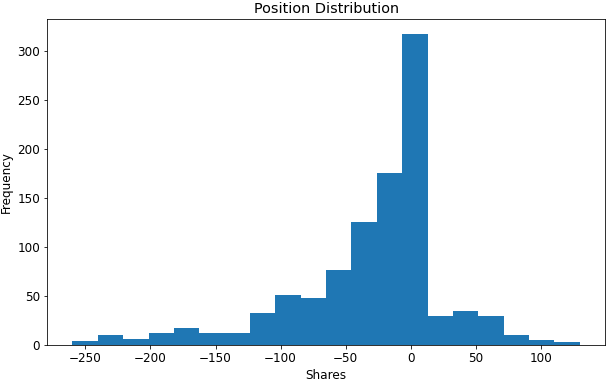
We can see the following from the preceding chart:
-
For this trading strategy, which has been applied to Google stock data, the strategy is
unlikely to have a position exceeding 200 shares(lower frequency) and has never had a position exceeding 250
. -
If it gets into position levels exceeding 250, we should be careful that the trading strategy is still performing as expected
.
Position holding time
While analyzing positions that a trading strategy gets into, it is also important to
measure how long a position stays open until it is
closed
and
returned to
its flat position
or
opposition position
. The longer a position stays open, the more risk it is taking on, because the more time there is for markets to make massive moves that can potentially
go against与…背道而驰
the open position.
A
long
position is initiated
开始实施,发起when the position goes from
- being short
- or flat
-
to being long
and
is closed
when the position goes back to
- flat
- or short.
Similarly,
short
positions are initiated
when the position goes from
- being long
- or flat
-
to being short
and
is closed
when the position goes back to
- flat
- or long.
Now, let’s find the distribution of open position durations with the help of the following code:
position_holding_times = []
current_pos = 0
current_pos_start = 0

for i in range(0, num_days):
    pos = results['Position'].iloc[i]

    # flat and starting a new position
    if current_pos ==0 : # current position = 0 after closing the position
        if pos !=0 :
            current_pos = pos
            current_pos_start = i
        continue
    # else:
    # going from long position to flat or short position or
    # going from short position to flat or long position
    if current_pos * pos <= 0: # +ve*(-ve)<0  and (+ve or -ve) * 0 =0
        position_holding_times.append( i-current_pos_start )
        current_pos = pos
        current_pos_start = i # new pos

print( position_holding_times )
figure = plt.figure( figsize=(10,6) )
plt.hist( position_holding_times, 100 )
plt.gca().set( title='Position Holding Time Distribution',
               xlabel='Holding time days',
               ylabel='Frequency'
             )
plt.show()
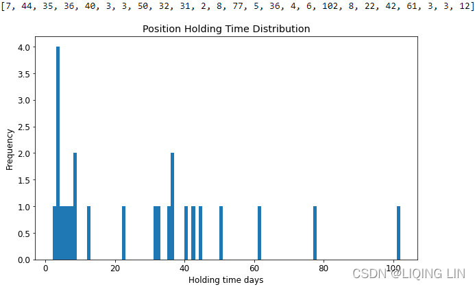
So, for this strategy, we can see that the holding time is pretty distributed, with
the longest one lasting around
102
days
and
the shortest one lasting around
3 days
.
Variance of PnLs
We need to measure
how much the PnLs can vary from day to day or even week to week
. This is an important measure of risk because if a trading strategy has large
swings
in PnLs, the account value is very
volatile
[ˈvɑːlətl]易变的,动荡不定的 and it is hard to run a trading strategy with such a profile. Often, we compute the
Standard Deviation of return
s
over different days or weeks or whatever timeframe we choose to use as our investment time horizon
. Most optimization methods try to
find optimal trading performance as a balance between PnLs and the Standard Deviation of returns
.
Computing the standard deviation of returns
is easy. Let’s compute the standard deviation of weekly returns, as shown in the following code:
last_week = 0
weekly_pnls = []

for i in range(0,num_days):

    if i - last_week >= 5:
        pnl_change = pnl[i] - pnl[last_week]
        weekly_pnls.append( pnl_change )

        last_week = i

from statistics import stdev, mean

print( 'PnL Standard Deviation:', stdev(weekly_pnls) )

figure = plt.figure( figsize=(10,6) )

plt.hist( weekly_pnls, 50 )
plt.gca().set( title='Weekly PnL Distribution',
               xlabel='$', ylabel='Frequency'
             )
plt.show()
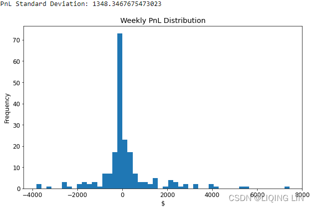
We can see that the
weekly PnLs are close to being
normally distributed around a mean of $0
, which intuitively makes sense.
The distribution is right skewed, which yields the positive cumulative PnLs for this trading strategy
.
There are some very large profits and losses for some weeks, but they are very rare, which is also within the expectations of what the distribution should look like
.
Sharpe ratio
Sharpe ratio is a very commonly used performance and risk metric that’s used in the industry to measure and compare the performance of algorithmic trading strategies.
Sharpe ratio
is defined as
the ratio of average PnL
over a period of time
and
the PnL standard deviation over the same period
. The benefit of the Sharpe ratio is that it
captures the profitability of a trading strategy
while
also accounting for the risk by using the volatility of the returns
. Let’s have a look at the mathematical representation:
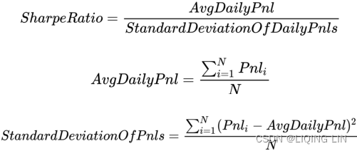
Here, we have the following:
-

: PnL on the

trading day. - N : Number of trading days over which this Sharpe is being computed.
Another performance and risk measure similar to the Sharpe ratio is known as the
Sortino ratio
, which
-
only uses observations where the trading strategy loses money
and
-
ignores the ones where the trading strategy makes money
.
The simple idea is that, for a trading strategy,
Sharpe upside moves in PnLs are a good thing, so they should not be considered when computing the standard deviation
.
Another way to say the same thing would be that
only downside moves or losses are actual risk observations
.
Let’s compute the
Sharpe and Sortino ratios
for our trading strategy. We will
use a week as the time horizon
for our trading strategy:
last_week_idx = 0
weekly_pnls = []
weekly_losses = []

for i in range(0, num_days):

    if i-last_week_idx >=5 :
        pnl_change = pnl[i] - pnl[last_week_idx]
        weekly_pnls.append( pnl_change )

        if pnl_change < 0:
            weekly_losses.append( pnl_change )

        last_week_idx = i

sharpe_ratio = mean( weekly_pnls ) / stdev(weekly_pnls)
sortino_ratio = mean( weekly_pnls ) / stdev(weekly_losses)

print( 'Sharpe ratio:', sharpe_ratio )
print( 'Sortion ratio:', sortino_ratio )
![]()
Here, we can see that
the Sharpe ratio and the Sortino ratio
are close to each other, which is what we expect since
both are risk-adjusted return metrics
. The
Sortino ratio is slightly higher than the Sharpe ratio
, which also makes sense since, by definition,
the Sortino ratio does not consider large increases in PnLs
as being contributions to the drawdown/risk for the trading strategy
, indicating that the
Sharpe ratio was
, in fact,
penalizing some large +ve jumps in PnLs
.
Maximum executions(or trades) per period
This risk measure is an
interval-based risk
check. An interval-based risk is
a counter that resets after a fixed amount of time and the risk check is imposed within such a time slice
. So, while
there is no final limit
, it’s important that
the limit isn’t exceeded within the time interval that is meant to detect and avoid over-trading
. The interval-based risk measure we will
inspect
is maximum executions per period
. This
measures
the maximum number of trades allowed in a given timeframe
. Then,
at the end of the timeframe, the counter is reset and starts over
. This would
detect and prevent
a runaway失控 strategy that buys and sells at a very fast pace
.
Let’s look at
the distribution of executions per period for our strategy using a week as our timeframe
, as shown here:
executions_this_week = 0
executions_per_week = []
last_week = 0

for i in range(0, num_days) :

    if results['Trades'].iloc[i] !=0 : # results['Trades']:[...,0,...,-1,...,1....]
        executions_this_week += 1

    if i-last_week >=5 :
        executions_per_week.append( executions_this_week )
        executions_this_week = 0
        last_week = i

figure = plt.figure( figsize=(10,6) )

plt.hist( executions_per_week, 10 )
plt.gca().set( title='Weekly number of executions Distribution',
               xlabel='Number of executions', ylabel='Frequency'
             )
plt.show()
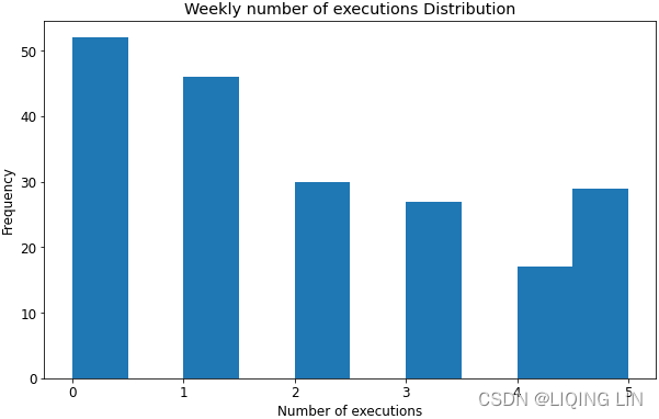
As we can see, for this trading strategy, it’s
never traded more than five times a week in the past
, which is when
it trades every day of the week
, which
doesn’t help us much
.
Now, let’s look at the maximum executions per month:
executions_this_month = 0
executions_per_month = []
last_month = 0

for i in range(0, num_days) :

    if results['Trades'].iloc[i] !=0 : # results['Trades']:[...,0,...,-1,...,1....]
        executions_this_month += 1

    if i-last_month >=20 :
        executions_per_month.append( executions_this_month )
        executions_this_month = 0
        last_month = i

figure = plt.figure( figsize=(10,6) )

plt.hist( executions_per_month, 10 )
plt.gca().set( title='Monthly number of executions Distribution',
               xlabel='Number of executions', ylabel='Frequency'
             )
plt.show()
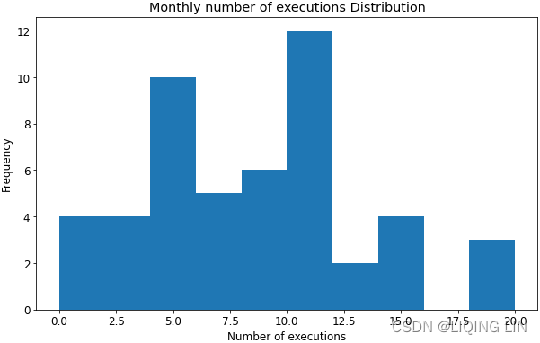
We can observe the following from the preceding plot:
-
It is possible for the strategy to trade every day in a month, so this risk measure can’t really be used for this strategy.
-
However, this is
still an important risk measure to understand and calibrate
, especially for algorithmic trading strategies that trade frequently, and especially for HFT strategies.
Maximum trade size
This risk metric measures what the
maximum possible trade size for a single trade
for the trading strategy is
. In our previous examples, we use
static trade sizes(-1,0 or 1)
, but it is not very difficult to build a trading strategy that
sends a larger order when the trading signal is stronger
and
a smaller order when the trading signal is weaker
. Alternatively, a strategy can choose to
liquidate a larger than normal position in one trade if it’s profitable
, in which case it will
send out a pretty large order
. This risk measure is also
very helpful when the trading strategy is a gray box trading strategy
as it
prevents fat-finger errors
, among other things. We will skip implementing this risk measure here, but
all we do is find a distribution of per trade size
, which should be straightforward to implement based on our implementation of previous risk measures.
Volume limits(Involving position changes)
This risk metric measures the traded volume, which
can also have an interval-based variant that measures volume
per period
. This is another risk measure that is meant to detect and prevent overtrading. For example, some of the catastrophic software implementation bugs we discussed in this chapter could’ve been prevented if they had a tight volume limit严格的交易量限制 in place that
warned operators about risk violations
and
possibly a volume limit that shut down trading strategies
.
Let’s observe the
traded volume
for our strategy, which is shown in the following code:
traded_volume = 0
for i in range(0, num_days):
    if results['Trades'].iloc[i] !=0 :
        traded_volume += abs( results['Position'].iloc[i] - results['Position'].iloc[i-1] )
print( 'Total traded volume:', traded_volume )
![]()
In this case, the strategy behavior is as expected, that is, no overtrading is detected. We can
use this to calibrate what total traded volume
to expect from this strategy
when it is deployed to live markets.
If it ever trades significantly more than what is expected, we can detect that to be an over-trading condition
.
Making a risk management algorithm
By now, we’re aware of the different types of risks and factors, including the risks in a trading strategy and the most common risk metrics for algorithmic trading strategies. Now, let’s have a look at
incorporating these risk measures into our volatility adjusted mean reversion trading strategy to make it safer before deploying it into live markets
. We will set the
risk limits to 150% of the maximum achieved historically
. We are doing this because it is possible that there is a day in the future that is very different from what we’ve seen historically. Let’s get started:
import pandas as pd
import pandas_datareader.data as pdr

def load_financial_data( start_date, end_date, output_file='', stock_symbol='GOOG' ):
    if len(output_file) == 0:
        output_file = stock_symbol+'_data_large.pkl'

    try:
        df = pd.read_pickle( output_file )
        print( "File {} data found...reading {} data".format( output_file ,stock_symbol) )
    except FileNotFoundError:
        print( "File {} not found...downloading the {} data".format( output_file, stock_symbol ) )
        df = pdr.DataReader( stock_symbol, "yahoo", start_date, end_date )
        df.to_pickle( output_file )
    return df

goog_data = load_financial_data( stock_symbol='GOOG',
                                 start_date='2014-01-01',
                                 end_date='2018-01-01',
                                 output_file='goog_data.pkl'
                               )
goog_data.head()

# Variables/constants for EMA Calculation:
NUM_PERIODS_FAST_10 = 10 # Static time period parameter for the fast EMA
K_FAST = 2/(NUM_PERIODS_FAST_10 + 1) # Static smoothing factor parameter for fast EMA
ema_fast = 0 # initial ema
ema_fast_values = [] # we will hold fast EMA values for visualization purpose

NUM_PERIODS_SLOW_40 = 40 # Static time period parameter for the slow EMA
K_SLOW = 2/(NUM_PERIODS_SLOW_40 + 1) # Static smoothing factor parameter for slow EMA
ema_slow = 0 # initial ema
ema_slow_values = [] # we will hold slow EMA values for visualization purpose

apo_values = [] # track computed absolute price oscillator values

# Variables for Trading Strategy trade, position & pnl management:

# Container for tracking buy/sell order,
# +1 for buy order, -1 for sell order, 0 for no-action
orders = []

# Container for tracking positions,
# positive for long positions, negative for short positions, 0 for flat/no position
positions = []

# Container for tracking total_pnls, this is the sum of
# closed_pnl i.e. pnls already locked in
# and open_pnl i.e. pnls for open-position marked to market price
pnls = []


last_buy_price = 0  # used to prevent over-trading at/around the same price
last_sell_price = 0 # used to prevent over-trading at/around the same price
position = 0 # Current position of the trading strategy

# Summation of products of
# buy_trade_price and buy_trade_qty for every buy Trade made
# since last time being flat
buy_sum_price_qty = 0
# Summation of buy_trade_qty for every buy Trade made since last time being flat
buy_sum_qty = 0

# Summation of products of
# sell_trade_price and sell_trade_qty for every sell Trade made
# since last time being flat
sell_sum_price_qty = 0
# Summation of sell_trade_qty for every sell Trade made since last time being flat
sell_sum_qty = 0

open_pnl = 0   # Open/Unrealized PnL marked to market
closed_pnl = 0 # Closed/Realized PnL so far

# Constants that define strategy behavior/thresholds

# APO trading signal value below which(-10) to enter buy-orders/long-position
APO_VALUE_FOR_BUY_ENTRY = -10 # (oversold, expect a bounce back up)
# APO trading signal value above which to enter sell-orders/short-position
APO_VALUE_FOR_SELL_ENTRY = 10 # (overbought, expect a bounce back down)

# Minimum price change since last trade before considering trading again,
MIN_PRICE_MOVE_FROM_LAST_TRADE = 10 # this is to prevent over-trading at/around same prices
NUM_SHARES_PER_TRADE = 10

# positions are closed if currently open positions are profitable above a certain amount,
# regardless of APO values.
# This is used to algorithmically lock profits and initiate more positions
# instead of relying only on the trading signal value.

# Minimum Open/Unrealized profit at which to close positions and lock profits
MIN_PROFIT_TO_CLOSE = 10*NUM_SHARES_PER_TRADE

import statistics as stats
import math as math

data3 = goog_data.copy()
close = data3['Close']

# Constants/variables that are used to compute standard deviation as a volatility measure
SMA_NUM_PERIODS_20 = 20 # look back period
price_history = []      # history of prices
1. Let’s define our risk limits, which we are not allowed to breach[briːtʃ]违反,破坏. As we discussed previously, it will be set to
150% of the historically observed maximums
# Risk limits
RISK_LIMIT_WEEKLY_STOP_LOSS = -7000*1.5 # -7000 from Weekly Loss Distribution
RISK_LIMIT_MONTHLY_STOP_LOSS = -8000*1.5 # -8000 from Monthly Loss Distribution
RISK_LIMIT_MAX_POSITION = 250*1.5       # 250( max( abs( short or long) ) from Position Distribution
RISK_LIMIT_MAX_POSITION_HOLDING_TIME_DAYS = 120*1.5 # 120 >105 from POSITION_HOLDING_TIME Distribution
RISK_LIMIT_MAX_TRADE_SIZE = 10*1.5 # NUM_SHARES_PER_TRADE = 10
RISK_LIMIT_MAX_TRADED_VOLUME = 4000*1.5 # 4000 from total trade volume limits
2. We will maintain some variables to
track and check for risk violations
with the help of the following code:
risk_violated = False

traded_volume = 0
current_pos = 0
current_pos_start = 0
3. As we can see, we have some code for computing the
Simple Moving Average
and
Standard Deviation for volatility adjustments
. We will compute
the fast and slow EMAs and the APO value
, which we can use as our
mean reversion(
prices revert toward the mean
) trading signal
:
# close = data3['Close']
for close_price in close:
    price_history.append( close_price )
    if len( price_history) > SMA_NUM_PERIODS_20 : # we track at most 'time_period' number of prices
        del ( price_history[0] )

    # calculate vairance during the SMA_NUM_PERIODS_20 periods
    sma = stats.mean( price_history )
    variance = 0 # variance is square of standard deviation
    for hist_price in price_history:
        variance = variance + ( (hist_price-sma)**2 )

    stddev = math.sqrt( variance/len(price_history) )

    # a volatility factor that ranges from 0 to 1
    stddev_factor = stddev/15 # 15 since since the population stddev.mean() = 15.45
    # closer to 0 indicate very low volatility,
    # around 1 indicate normal volatility
    # > 1 indicate above-normal volatility
    if stddev_factor == 0:
        stddev_factor = 1

    # This section updates fast and slow EMA and computes APO trading signal
    if (ema_fast==0): # first observation
        ema_fast = close_price # initial ema_fast or ema_slow
        ema_slow = close_price
    else:
        # ema fomula
        # K_FAST*stddev_factor or K_SLOW*stddev_factor
        # more reactive to newest observations during periods of higher than normal volatility
        ema_fast = (close_price-ema_fast) * K_FAST*stddev_factor + ema_fast
        ema_slow = (close_price-ema_slow) * K_SLOW*stddev_factor + ema_slow

    ema_fast_values.append( ema_fast )
    ema_slow_values.append( ema_slow )

    apo = ema_fast - ema_slow
    apo_values.append( apo )

    ############################
    # 4.# Now, before we can evaluate our signal and
    #     check whether we can send an order out,
    #     we need to perform a risk check to ensure that the trade size we may attempt
    #   # is within MAX_TRADE_SIZE limits:
    if NUM_SHARES_PER_TRADE > RISK_LIMIT_MAX_TRADE_SIZE :
        print( 'Risk Violation: NUM_SHARES_PER_TRADE', NUM_SHARES_PER_TRADE,
               ' > RISK_LIMIT_MAX_TRADE_SIZE', RISK_LIMIT_MAX_TRADE_SIZE
             )
        risk_violated=True
    ############################

    # 6. This section checks trading signal against trading parameters/thresholds and positions, to trade.

    # We will perform a sell trade at close_price if the following conditions are met:
    # 1. The APO trading signal value(positive) > Sell-Entry threshold (overbought, expect a bounce back down, sell for profit)
    #     and the difference between current-price and last trade-price is different enough.(>Minimum price change)
    # 2. We are long( +ve position ) and
    #    either APO trading signal value >= 0 or current position is profitable enough to lock profit.
    # APO_VALUE_FOR_SELL_ENTRY * stdev_factor:
    #              by increasing the threshold for entry by a factor of volatility,
    #              makes us less aggressive in entering positions(here is sell) during periods of higher volatility,
    # dynamic MIN_PROFIT_TO_CLOSE / stddev_factor:
    #              to decrease the the expected profit threshold during periods of increased volatility
    #              to be more aggressive in exciting positions
    #              it is riskier to hold on to positions for longer periods of time.
    if not risk_violated and ( ( apo > APO_VALUE_FOR_SELL_ENTRY*stddev_factor and \
                                 abs( close_price-last_sell_price ) > MIN_PRICE_MOVE_FROM_LAST_TRADE*stddev_factor
                               )
                               or
                               ( position>0 and (apo >=0 or open_pnl > MIN_PROFIT_TO_CLOSE/stddev_factor ) )
                             ): # long from -ve APO and APO has gone positive or position is profitable, sell to close position
        orders.append(-1) # mark the sell trade
        last_sell_price = close_price
        position -= NUM_SHARES_PER_TRADE
        traded_volume += NUM_SHARES_PER_TRADE ############################
        sell_sum_qty += NUM_SHARES_PER_TRADE
        sell_sum_price_qty += (close_price * NUM_SHARES_PER_TRADE) # update vwap sell-price
        print( "Sell ", NUM_SHARES_PER_TRADE, " @ ", close_price, "Position: ", position )

    # 7. We will perform a buy trade at close_price if the following conditions are met:
    # 1. The APO trading signal value(negative) < below Buy-Entry threshold (oversold, expect a bounce back up, buy for future profit)
    #    and the difference between current-price and last trade-price is different enough.(>Minimum price change)
    # 2. We are short( -ve position ) and
    #    either APO trading signal value is <= 0 or current position is profitable enough to lock profit.
    # APO_VALUE_FOR_BUY_ENTRY * stdev_factor:
    #              by increasing the threshold for entry by a factor of volatility,
    #              makes us less aggressive in entering positions(here is sell) during periods of higher volatility,
    # dynamic MIN_PROFIT_TO_CLOSE / stddev_factor:
    #              to decrease the the expected profit threshold during periods of increased volatility
    #              to be more aggressive in exciting positions
    #              it is riskier to hold on to positions for longer periods of time.
    elif not risk_violated and ( ( apo < APO_VALUE_FOR_BUY_ENTRY*stddev_factor and \
                                   abs( close_price-last_buy_price ) > MIN_PRICE_MOVE_FROM_LAST_TRADE*stddev_factor
                                 )
                                 or
                                 ( position<0 and (apo <=0 or open_pnl > MIN_PROFIT_TO_CLOSE/stddev_factor ) )
                               ): # short from +ve APO and APO has gone negative or position is profitable, buy to close position
        orders.append(+1) # mark the buy trade
        last_buy_price = close_price
        position += NUM_SHARES_PER_TRADE
        traded_volume += NUM_SHARES_PER_TRADE ############################
        buy_sum_qty += NUM_SHARES_PER_TRADE
        buy_sum_price_qty += (close_price * NUM_SHARES_PER_TRADE) # update the vwap buy-price
        print( "Buy ", NUM_SHARES_PER_TRADE, " @ ", close_price, "Position: ", position )
    else:
        # No trade since none of the conditions were met to buy or sell
        orders.append( 0 )

    positions.append( position )

    ############################
    # 6.# Now, we will check that, after any potential orders have been sent out and trades
    #     have been made this round, we haven't breached any of our risk limits,
    #   # starting with the Maximum Position Holding Time risk limit.
    # flat and starting a new postion
    if current_pos ==0 : # current position = 0 after closing the position
        if position != 0:
            current_pos = position
            current_pos_start = len(positions) # new start index

    # going from long position to flat or short position or
    # going from short position to flat or long position
    elif current_pos * position <=0 :
        position_holding_time = len(positions) - current_pos_start
        current_pos = position
        current_pos_start = len(positions)

        if position_holding_time > RISK_LIMIT_MAX_POSITION_HOLDING_TIME_DAYS:
            print( 'Risk Violation: position_holding_time', position_holding_time,
                   ' > RISK_LIMIT_MAX_POSITION_HOLDING_TIME_DAYS', RISK_LIMIT_MAX_POSITION_HOLDING_TIME_DAYS
                 )
            risk_violated = True

    # 7. check that the new long/short position is within the Max Position risk limits
    if abs(position) > RISK_LIMIT_MAX_POSITION:
        print( 'Risk Violation: position', position,
               ' > RISK_LIMIT_MAX_POSITION', RISK_LIMIT_MAX_POSITION
             )
    # 8. check that the updated traded volume doesn't violate the allocated Maximum Traded Volume risk limit:
    if traded_volume  > RISK_LIMIT_MAX_TRADED_VOLUME:
        print( 'Risk Violation: traded_volume', traded_volume,
               ' > RISK_LIMIT_MAX_TRADED_VOLUME', RISK_LIMIT_MAX_TRADED_VOLUME
             )
        risk_violated = True
    ############################

    # 8. The code of the trading strategy contains logic for position/PnL management.
    #    It needs to update positions and compute open and closed PnLs when market prices change
    #    and/or trades are made causing a change in positions

    # This section updates Open/Unrealized & Closed/Realized positions
    open_pnl = 0
    if position > 0:
        # long position and some sell trades have been made against it,
        # close that amount based on how much was sold against this long position
        # PnL_realized = sell_sum_qty * (Average Sell Price - Average Buy Price)
        if sell_sum_qty > 0:           # vwap for sell                   # vwap  for buy
            open_pnl = sell_sum_qty * (sell_sum_price_qty/sell_sum_qty - buy_sum_price_qty/buy_sum_qty)
        # mark the remaining position to market
        # i.e. pnl would be what it would be if we closed at current price
        # sell
        # position -= NUM_SHARES_PER_TRADE
        # sell_sum_qty += NUM_SHARES_PER_TRADE
        # PnL_unrealized = remaining position * (Exit Price - Average Buy Price)
        # if now, sell sell_sum_qty @ any price, we should use abs(position-sell_sum_qty) *
        open_pnl += abs(position) * ( close_price - buy_sum_price_qty/buy_sum_qty )
        # print( position, (buy_sum_qty-sell_sum_qty), open_pnl)
    elif position < 0:
        # short position and some buy trades have been made against it,
        # close that amount based on how much was bought against this short position
        # PnL_realized = buy_sum_qty * (Average Sell Price - Average Buy Price)
        if buy_sum_qty > 0:           # vwap for sell                   # vwap  for buy
            open_pnl = buy_sum_qty * (sell_sum_price_qty/sell_sum_qty - buy_sum_price_qty/buy_sum_qty)
        # mark the remaining position to market
        # i.e. pnl would be what it would be if we closed at current price
        # buy
        # position += NUM_SHARE_PER_TRADE
        # buy_sum_qty += NUM_SHARE_PER_TRADE
        # PnL_unrealized = remaining position * (Average Sell Price - Exit Price)
        # if now, buy buy_sum_qty @ any price, we should use abs(position+buy_sum_qty) *
        open_pnl += abs(position) * ( sell_sum_price_qty/sell_sum_qty - close_price )
        # print( position, (buy_sum_qty-sell_sum_qty), open_pnl)
    else:
        # flat, so update closed_pnl and reset tracking variables for positions & pnls
        closed_pnl += (sell_sum_price_qty - buy_sum_price_qty)

        buy_sum_price_qty = 0
        buy_sum_qty = 0
        last_buy_price = 0

        sell_sum_price_qty = 0
        sell_sum_qty = 0
        last_sell_price = 0

    print( "OpenPnL: ", open_pnl, " ClosedPnL: ", closed_pnl, " TotalPnL: ", (open_pnl + closed_pnl) )
    pnls.append(closed_pnl + open_pnl)

    ############################
    if len( pnls ) > 5:
        weekly_loss = pnls[-1] - pnls[-6] # negative value

        if weekly_loss < RISK_LIMIT_WEEKLY_STOP_LOSS:
            print( 'Risk Violation : weekly_loss', week_loss,
                   ' < RISK_LIMIT_WEEKLY_STOP_LOSS', RISK_LIMIT_WEEKLY_STOP_LOSS
                 )
            risk_violated = True

    if len( pnls ) > 20:
        monthly_loss = pnls[-1] - pnls[-21]

        if monthly_loss < RISK_LIMIT_MONTHLY_STOP_LOSS:
            print( 'Risk Violation : monthly_loss', monthly_loss,
                   '< RISK_LIMIT_MONTHLY_STOP_LOSS', RISK_LIMIT_MONTHLY_STOP_LOSS
                 )
            risk_violated = True

    ############################
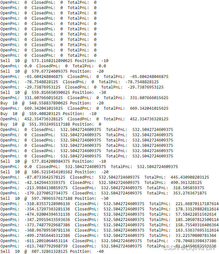
Here, we
have added a robust risk management system to our existing trading strategy that can be extended to any other trading strategies
we intend on deploying to live trading markets in the future. This will
protect live trading strategies from going rogue[roʊɡ]流氓 in production or behaving outside of our expected parameters
, hence providing great risk control over our trading strategies.
# This section prepares the dataframe from the trading strategy results and visualizes the results
data3 = data3.assign( ClosePrice = pd.Series(close, index=data3.index) )
data3 = data3.assign( Fast10DayEMA = pd.Series(ema_fast_values, index=data3.index) )
data3 = data3.assign( Slow40DayEMA = pd.Series(ema_slow_values, index=data3.index) )
data3 = data3.assign( APO = pd.Series(apo_values, index=data3.index) )
data3 = data3.assign( Trades = pd.Series(orders, index=data3.index) )
data3 = data3.assign( Position = pd.Series(positions, index=data3.index) )
data3 = data3.assign( Pnl = pd.Series(pnls, index=data3.index) )
import matplotlib.pyplot as plt
fig = plt.figure( figsize=(20,10) )
data3['ClosePrice'].plot(color='k', lw=3., legend=True)
data3['Fast10DayEMA'].plot(color='y', lw=1., legend=True)
data3['Slow40DayEMA'].plot(color='m', lw=1., legend=True)
plt.plot( data3.loc[ data3.Trades == 1 ].index, data3.ClosePrice[data3.Trades == 1 ],
color='y', lw=0, marker='^', markersize=7, label='buy'
)
plt.plot( data3.loc[ data3.Trades == -1 ].index, data3.ClosePrice[data3.Trades == -1 ],
color='b', lw=0, marker='v', markersize=7, label='sell'
)
plt.autoscale(enable=True, axis='x', tight=True)
plt.legend()
plt.show()
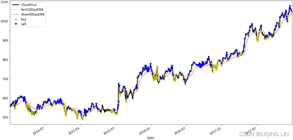
This result is the same as before, because the limitation is based on historical data, no new data is added.
fig = plt.figure( figsize=(20,10) )

data3['Pnl'].plot(color='k', lw=1., legend=True)
plt.plot( data3.loc[ data3.Pnl > 0 ].index, data3.Pnl[ data3.Pnl > 0 ],
          color='b', lw=0, marker='.'
        )
plt.plot( data3.loc[ data3.Pnl < 0 ].index, data3.Pnl[ data3.Pnl < 0 ],
         color='r', lw=0, marker='.'
        )

plt.autoscale( enable=True, axis='x', tight=True)
plt.legend()
plt.show()
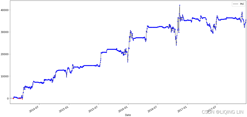
Realistically adjusting risk
In the risk management system we built in the previous section, we used
static risk limits
that we used for the duration of the strategy’s lifetime. In practice, however, this is never the case.
When
a new algorithmic trading strategy
is built and deployed, it is
first deployed with
very low-risk limits
—usually
the least amount of risk
possible
. This is for a variety of
reasons
,
-
the
first
one being to
make tests and work out software implementation bugs
, if there are any.
The larger the amount of new code being deployed to live markets, the greater the risk
. -
The other reason
is to make sure
strategy behavior is consistent with what is expected based on historical performance analysis
.-
It is usually
monitored
very closely by
multiple people
to make sure
nothing unexpected happens
. -
Then, after a couple of days or weeks, when
initial bugs
have been worked out
and
strategy performance
is in line with
simulation performance
,
it is slowly scaled up to
take more risks
in order to
generate more profits
.
-
It is usually
Conversely, after a strategy goes through a bad patch of losses, it is often
reevaluated
at
reduced risk limits
to
check
whether the trading strategy’s performance has degraded from historical expectations
and
if it is no longer profitable to deploy it in live markets anymore
.
The obvious objective is to make as much money as possible, but achieving that requires
not only a good risk check system but also a good system to
adjust risk through different PnL profiles
in the lifetime of the strategy
.
A simple intuitive approach to adjusting risk in trading can be to
start with low risk
,
increase the risk slightly after a good performance
, and
reduce the risk slightly after a poor performance
. This is generally the approach that’s followed by most participants: the challenges are to
quantify good/poor performance in order to increase/decrease risk and to quantify the amount by which to increase/decrease risk
.
import pandas as pd
import pandas_datareader.data as pdr

def load_financial_data( start_date, end_date, output_file='', stock_symbol='GOOG' ):
    if len(output_file) == 0:
        output_file = stock_symbol+'_data_large.pkl'

    try:
        df = pd.read_pickle( output_file )
        print( "File {} data found...reading {} data".format( output_file ,stock_symbol) )
    except FileNotFoundError:
        print( "File {} not found...downloading the {} data".format( output_file, stock_symbol ) )
        df = pdr.DataReader( stock_symbol, "yahoo", start_date, end_date )
        df.to_pickle( output_file )
    return df

goog_data = load_financial_data( stock_symbol='GOOG',
                                 start_date='2014-01-01',
                                 end_date='2018-01-01',
                                 output_file='goog_data.pkl'
                               )
goog_data.head()

# Variables/constants for EMA Calculation:
NUM_PERIODS_FAST_10 = 10 # Static time period parameter for the fast EMA
K_FAST = 2/(NUM_PERIODS_FAST_10 + 1) # Static smoothing factor parameter for fast EMA
ema_fast = 0 # initial ema
ema_fast_values = [] # we will hold fast EMA values for visualization purpose

NUM_PERIODS_SLOW_40 = 40 # Static time period parameter for the slow EMA
K_SLOW = 2/(NUM_PERIODS_SLOW_40 + 1) # Static smoothing factor parameter for slow EMA
ema_slow = 0 # initial ema
ema_slow_values = [] # we will hold slow EMA values for visualization purpose

apo_values = [] # track computed absolute price oscillator values

# Variables for Trading Strategy trade, position & pnl management:

# Container for tracking buy/sell order,
# +1 for buy order, -1 for sell order, 0 for no-action
orders = []

# Container for tracking positions,
# positive for long positions, negative for short positions, 0 for flat/no position
positions = []

# Container for tracking total_pnls, this is the sum of
# closed_pnl i.e. pnls already locked in
# and open_pnl i.e. pnls for open-position marked to market price
pnls = []


last_buy_price = 0  # used to prevent over-trading at/around the same price
last_sell_price = 0 # used to prevent over-trading at/around the same price
position = 0 # Current position of the trading strategy

# Summation of products of
# buy_trade_price and buy_trade_qty for every buy Trade made
# since last time being flat
buy_sum_price_qty = 0
# Summation of buy_trade_qty for every buy Trade made since last time being flat
buy_sum_qty = 0

# Summation of products of
# sell_trade_price and sell_trade_qty for every sell Trade made
# since last time being flat
sell_sum_price_qty = 0
# Summation of sell_trade_qty for every sell Trade made since last time being flat
sell_sum_qty = 0

open_pnl = 0   # Open/Unrealized PnL marked to market
closed_pnl = 0 # Closed/Realized PnL so far

# Constants that define strategy behavior/thresholds

# APO trading signal value below which(-10) to enter buy-orders/long-position
APO_VALUE_FOR_BUY_ENTRY = -10 # (oversold, expect a bounce back up)
# APO trading signal value above which to enter sell-orders/short-position
APO_VALUE_FOR_SELL_ENTRY = 10 # (overbought, expect a bounce back down)

# Minimum price change since last trade before considering trading again,
MIN_PRICE_MOVE_FROM_LAST_TRADE = 10 # this is to prevent over-trading at/around same prices
Let’s look at a practical implementation using our previous
volatility adjusted mean reversion strategy
with risk checks
. We will
increase the trade size and risk after a good month and reduce the trade size and risk after a bad month by a small increment
. Let’s get started:
1.
First, we will
define the limits
of
how small a trade size can be and what the maximum allowed trade size
can be over the course of the strategy’s lifetime. For this implementation, we allow
no less than 5 share per trade and no more than 50 per trade
. Every time we have a good/bad month, we will
increase/decrease the trade size by 5 shares
. We will start very small, as we discussed previously, and increment slowly if we continue to do well. Let’s have a look at the code:
MIN_NUM_SHARES_PER_TRADE = 5       ### Influence PnL
MAX_NUM_SHARES_PER_TRADE = 50
INCREMENT_NUM_SHARES_PER_TRADE = 5 ###
num_shares_per_trade = MIN_NUM_SHARES_PER_TRADE # Beginning number of shares to buy/sell on every trade
num_shares_history = []   # history of num-shares
abs_position_history = [] # history of absolute-position
import statistics as stats
import math as math
# Constants/variables that are used to compute standard deviation as a volatility measure
SMA_NUM_PERIODS_20 = 20 # look back period
price_history = [] # history of prices
2.
Next, we will define similar
minimum, maximum, and increment values for the different risk limits
. As the
strategy
trade size
evolves over time, the risk limits will also have to be adjusted to accommodate the increased
trading size
:
# Risk limits and increments to risk limits when we have good/bad months
risk_limit_weekly_stop_loss = -500
INCREMENT_RISK_LIMIT_WEEKLY_STOP_LOSS = -1000 # -7000 from Weekly Loss Distribution
# INCREMENT_RISK_LIMIT_WEEKLY_STOP_LOSS = -12000

risk_limit_monthly_stop_loss = -2000 # 20/5=4*(-500)=-2000
INCREMENT_RISK_LIMIT_MONTHLY_STOP_LOSS = -1000
# risk_limit_monthly_stop_loss = -15000
# INCREMENT_RISK_LIMIT_MONTHLY_STOP_LOSS = -30000

risk_limit_max_position = 100           ######
INCREMENT_RISK_LIMIT_MAX_POSITION = 20  ######

max_position_history = [] # history of max-trade-size
RISK_LIMIT_MAX_POSITION_HOLDING_TIME_DAYS = 120

risk_limit_max_trade_size = 20
INCREMENT_RISK_LIMIT_MAX_TRADE_SIZE = 5
max_trade_size_history = [] # history of max-trade-size

risk_violated = False

traded_volume = 0
current_pos = 0
current_pos_start = 0

last_risk_change_index = 0  #######
data4 = goog_data.copy()
close = data4['Close']
for close_price in close:
price_history.append( close_price )
if len( price_history) > SMA_NUM_PERIODS_20 : # we track at most 'time_period' number of prices
del ( price_history[0] )
# calculate vairance during the SMA_NUM_PERIODS_20 periods
sma = stats.mean( price_history )
variance = 0 # variance is square of standard deviation
for hist_price in price_history:
variance = variance + ( (hist_price-sma)**2 )
stddev = math.sqrt( variance/len(price_history) )
# a volatility factor that ranges from 0 to 1
stddev_factor = stddev/15 # 15 since since the population stddev.mean() = 15.45
# closer to 0 indicate very low volatility,
# around 1 indicate normal volatility
# > 1 indicate above-normal volatility
if stddev_factor == 0:
stddev_factor = 1
# This section updates fast and slow EMA and computes APO trading signal
if (ema_fast==0): # first observation
ema_fast = close_price # initial ema_fast or ema_slow
ema_slow = close_price
else:
# ema fomula
# K_FAST*stddev_factor or K_SLOW*stddev_factor
# more reactive to newest observations during periods of higher than normal volatility
ema_fast = (close_price-ema_fast) * K_FAST*stddev_factor + ema_fast
ema_slow = (close_price-ema_slow) * K_SLOW*stddev_factor + ema_slow
ema_fast_values.append( ema_fast )
ema_slow_values.append( ema_slow )
apo = ema_fast - ema_slow
apo_values.append( apo )
############################
# 4.# Now, before we can evaluate our signal and
# check whether we can send an order out,
# we need to perform a risk check to ensure that the trade size we may attempt
# # is within MAX_TRADE_SIZE limits:
if num_shares_per_trade > risk_limit_max_trade_size :
print( 'Risk Violation: NUM_SHARES_PER_TRADE', num_shares_per_trade,
' > RISK_LIMIT_MAX_TRADE_SIZE', risk_limit_max_trade_size
)
risk_violated=True
MIN_PROFIT_TO_CLOSE = num_shares_per_trade * 10
############################
# 6. This section checks trading signal against trading parameters/thresholds and positions, to trade.
# We will perform a sell trade at close_price if the following conditions are met:
# 1. The APO trading signal value(positive) > Sell-Entry threshold (overbought, expect a bounce back down, sell for profit)
# and the difference between current-price and last trade-price is different enough.(>Minimum price change)
# 2. We are long( +ve position ) and
# either APO trading signal value >= 0 or current position is profitable enough to lock profit.
# APO_VALUE_FOR_SELL_ENTRY * stdev_factor:
# by increasing the threshold for entry by a factor of volatility,
# makes us less aggressive in entering positions(here is sell) during periods of higher volatility,
# dynamic MIN_PROFIT_TO_CLOSE / stddev_factor:
# to decrease the the expected profit threshold during periods of increased volatility
# to be more aggressive in exciting positions
# it is riskier to hold on to positions for longer periods of time.
if not risk_violated and ( ( apo > APO_VALUE_FOR_SELL_ENTRY*stddev_factor and \
abs( close_price-last_sell_price ) > MIN_PRICE_MOVE_FROM_LAST_TRADE*stddev_factor
)
or
( position>0 and (apo >=0 or open_pnl > MIN_PROFIT_TO_CLOSE/stddev_factor ) )
): # long from -ve APO and APO has gone positive or position is profitable, sell to close position
orders.append(-1) # mark the sell trade
last_sell_price = close_price
############################
if (-risk_limit_max_position)< position<=0: # opening a new entry position
position -= num_shares_per_trade # reduce position by the size of this trade
traded_volume += num_shares_per_trade
sell_sum_qty += num_shares_per_trade
sell_sum_price_qty += (close_price * num_shares_per_trade) # update vwap sell-price
print( "Sell ", num_shares_per_trade, " @ ", close_price, "Position: ", position )
elif position >0: # closing an existing position, position < 0?
traded_volume += abs(position)
sell_sum_qty += abs(position)
sell_sum_price_qty += (close_price * abs(position) ) # update vwap sell-price
print( "Sell ", abs(position), " @ ", close_price, "Position: ", position )
position = 0
else:#elif abs(position) > risk_limit_max_position:
print( 'Risk Violation: position', position,
' > RISK_LIMIT_MAX_POSITION', risk_limit_max_position
)
traded_volume += abs(position)
buy_sum_qty += abs(position)
buy_sum_price_qty += (close_price * abs(position) ) # update vwap sell-price
print( "Buy ", abs(position), " @ ", close_price, "Position: ", position )
position = 0
############################
# 7. We will perform a buy trade at close_price if the following conditions are met:
# 1. The APO trading signal value(negative) < below Buy-Entry threshold (oversold, expect a bounce back up, buy for future profit)
# and the difference between current-price and last trade-price is different enough.(>Minimum price change)
# 2. We are short( -ve position ) and
# either APO trading signal value is <= 0 or current position is profitable enough to lock profit.
# APO_VALUE_FOR_BUY_ENTRY * stdev_factor:
# by increasing the threshold for entry by a factor of volatility,
# makes us less aggressive in entering positions(here is sell) during periods of higher volatility,
# dynamic MIN_PROFIT_TO_CLOSE / stddev_factor:
# to decrease the the expected profit threshold during periods of increased volatility
# to be more aggressive in exciting positions
# it is riskier to hold on to positions for longer periods of time.
elif not risk_violated and ( ( apo < APO_VALUE_FOR_BUY_ENTRY*stddev_factor and \
abs( close_price-last_buy_price ) > MIN_PRICE_MOVE_FROM_LAST_TRADE*stddev_factor
)
or
( position<0 and (apo <=0 or open_pnl > MIN_PROFIT_TO_CLOSE/stddev_factor ) )
): # short from +ve APO and APO has gone negative or position is profitable, buy to close position
orders.append(+1) # mark the buy trade
last_buy_price = close_price
############################
if 0 <= position < risk_limit_max_position: # opening a new entry position
position += num_shares_per_trade
traded_volume += num_shares_per_trade
buy_sum_qty += num_shares_per_trade
buy_sum_price_qty += (close_price * num_shares_per_trade) # update the vwap buy-price
print( "Buy ", num_shares_per_trade, " @ ", close_price, "Position: ", position )
elif position<0:# position<0 : # position <0, closing an existing position
traded_volume += abs(position)
buy_sum_qty += abs(position)
buy_sum_price_qty += (close_price * abs(position)) # update the vwap buy-price
print( "Buy ", abs(position), " @ ", close_price, "Position: ", position )
position = 0 # increase position by the size of this trade
else: #elif abs(position) > risk_limit_max_position:
print( 'Risk Violation: position', position,
' > RISK_LIMIT_MAX_POSITION', risk_limit_max_position
)
traded_volume += abs(position)
sell_sum_qty += abs(position)
sell_sum_price_qty += (close_price * abs(position)) # update the vwap buy-price
print( "Sell ", abs(position), " @ ", close_price, "Position: ", position )
position = 0 # increase position by the size of this trade
############################
else:
# No trade since none of the conditions were met to buy or sell
orders.append( 0 )
positions.append( position )
############################
# 6.# Now, we will check that, after any potential orders have been sent out and trades
# have been made this round, we haven't breached any of our risk limits,
# # starting with the Maximum Position Holding Time risk limit.
# flat and starting a new postion
if current_pos ==0 : # current position = 0 after closing the position
if position != 0:
current_pos = position
current_pos_start = len(positions) # new start index
# going from long position to flat or short position or
# going from short position to flat or long position
elif current_pos * position <=0 :
position_holding_time = len(positions) - current_pos_start
current_pos = position
current_pos_start = len(positions)
if position_holding_time > RISK_LIMIT_MAX_POSITION_HOLDING_TIME_DAYS:
print( 'Risk Violation: position_holding_time', position_holding_time,
' > RISK_LIMIT_MAX_POSITION_HOLDING_TIME_DAYS', RISK_LIMIT_MAX_POSITION_HOLDING_TIME_DAYS
)
risk_violated = True
# # 7. check that the new long/short position is within the Max Position risk limits
# if abs(position) > risk_limit_max_position:
# print( 'Risk Violation: position', position,
# ' > RISK_LIMIT_MAX_POSITION', risk_limit_max_position
# )
# risk_violated = True
############################
# 8. The code of the trading strategy contains logic for position/PnL management.
# It needs to update positions and compute open and closed PnLs when market prices change
# and/or trades are made causing a change in positions
# This section updates Open/Unrealized & Closed/Realized positions
open_pnl = 0
if position > 0: # after -sell_sum_qty
# long position and some sell trades have been made against it,
# close that amount based on how much was sold against this long position
# PnL_realized = sell_sum_qty * (Average Sell Price - Average Buy Price)
if sell_sum_qty > 0: # vwap for sell # vwap for buy
open_pnl = sell_sum_qty * (sell_sum_price_qty/sell_sum_qty - buy_sum_price_qty/buy_sum_qty)
# mark the remaining position to market
# i.e. pnl would be what it would be if we closed at current price
# sell
# position -= NUM_SHARES_PER_TRADE
# sell_sum_qty += NUM_SHARES_PER_TRADE
# PnL_unrealized = remaining position * (Exit Price - Average Buy Price)
# if now, sell sell_sum_qty @ any price, we should use abs(position-sell_sum_qty) *
open_pnl += abs(position) * ( close_price - buy_sum_price_qty/buy_sum_qty )
# print( position, (buy_sum_qty-sell_sum_qty), open_pnl)
elif position < 0: # # after +buy_sum_qty
# short position and some buy trades have been made against it,
# close that amount based on how much was bought against this short position
# PnL_realized = buy_sum_qty * (Average Sell Price - Average Buy Price)
if buy_sum_qty > 0: # vwap for sell # vwap for buy
open_pnl = buy_sum_qty * (sell_sum_price_qty/sell_sum_qty - buy_sum_price_qty/buy_sum_qty)
# mark the remaining position to market
# i.e. pnl would be what it would be if we closed at current price
# buy
# position += NUM_SHARE_PER_TRADE
# buy_sum_qty += NUM_SHARE_PER_TRADE
# PnL_unrealized = remaining position * (Average Sell Price - Exit Price)
# if now, buy buy_sum_qty @ any price, we should use abs(position+buy_sum_qty) *
open_pnl += abs(position) * ( sell_sum_price_qty/sell_sum_qty - close_price )
# print( position, (buy_sum_qty-sell_sum_qty), open_pnl)
else:
# flat, so update closed_pnl and reset tracking variables for positions & pnls
closed_pnl += (sell_sum_price_qty - buy_sum_price_qty)
buy_sum_price_qty = 0
buy_sum_qty = 0
last_buy_price = 0
sell_sum_price_qty = 0
sell_sum_qty = 0
last_sell_price = 0
print( "OpenPnL: ", open_pnl, " ClosedPnL: ", closed_pnl, " TotalPnL: ", (open_pnl + closed_pnl) )
pnls.append(closed_pnl + open_pnl)
############################
# Analyze monthly performance and adjust risk up/down
if len( pnls ) > 20:
monthly_pnls = pnls[-1] - pnls[-21]
if len(pnls) - last_risk_change_index > 20:
# increase trade size and risk limits if we had a good month
if monthly_pnls > 0:
num_shares_per_trade += INCREMENT_NUM_SHARES_PER_TRADE
if num_shares_per_trade <= MAX_NUM_SHARES_PER_TRADE :
print( 'Increasing trade-size and risk' )
risk_limit_weekly_stop_loss += INCREMENT_RISK_LIMIT_WEEKLY_STOP_LOSS
risk_limit_monthly_stop_loss += INCREMENT_RISK_LIMIT_MONTHLY_STOP_LOSS
risk_limit_max_position += INCREMENT_RISK_LIMIT_MAX_POSITION
risk_limit_max_trade_size += INCREMENT_RISK_LIMIT_MAX_TRADE_SIZE
else:
num_shares_per_trade = MAX_NUM_SHARES_PER_TRADE
# decrease trade size and risk limits if we had a bad month
elif monthly_pnls < 0:
num_shares_per_trade -= INCREMENT_NUM_SHARES_PER_TRADE
if num_shares_per_trade >= MIN_NUM_SHARES_PER_TRADE :
print('Decreasing trade-size and risk')
risk_limit_weekly_stop_loss -= INCREMENT_RISK_LIMIT_WEEKLY_STOP_LOSS
risk_limit_monthly_stop_loss -= INCREMENT_RISK_LIMIT_MONTHLY_STOP_LOSS
risk_limit_max_position -= INCREMENT_RISK_LIMIT_MAX_POSITION
risk_limit_max_trade_size -= INCREMENT_RISK_LIMIT_MAX_TRADE_SIZE
else:
num_shares_per_trade = MIN_NUM_SHARES_PER_TRADE
last_risk_change_index = len(pnls)
# end if len( pnls ) > 20
# Track trade-sizes/positions and risk limits as they evolve over time
num_shares_history.append( num_shares_per_trade )
abs_position_history.append( abs(position) )
max_trade_size_history.append( risk_limit_max_trade_size )
max_position_history.append( risk_limit_max_position )
if len( pnls ) > 5:
weekly_loss = pnls[-1] - pnls[-6] # negative value
if weekly_loss < risk_limit_weekly_stop_loss:
print( 'Risk Violation : weekly_loss', weekly_loss,
' < RISK_LIMIT_WEEKLY_STOP_LOSS', risk_limit_weekly_stop_loss
)
risk_violated = True
if len( pnls ) > 20:
monthly_loss = pnls[-1] - pnls[-21]
if monthly_loss < risk_limit_monthly_stop_loss:
print( 'Risk Violation : monthly_loss', monthly_loss,
'< RISK_LIMIT_MONTHLY_STOP_LOSS', risk_limit_monthly_stop_loss
)
risk_violated = True
############################
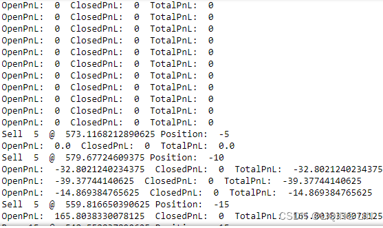
… …
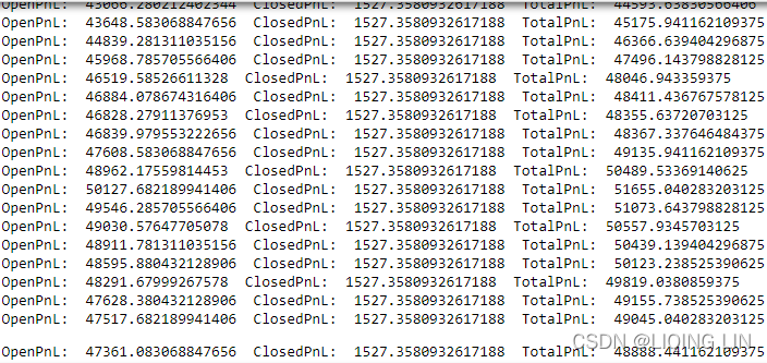
# This section prepares the dataframe from the trading strategy results and visualizes the results
data4 = data4.assign( ClosePrice=pd.Series(close, index=data4.index) )
data4 = data4.assign( Fast10DayEMA=pd.Series(ema_fast_values, index=data4.index) )
data4 = data4.assign( Slow40DayEMA=pd.Series(ema_slow_values, index=data4.index) )
data4 = data4.assign( APO=pd.Series(apo_values, index=data4.index) )
data4 = data4.assign( Trades=pd.Series(orders, index=data4.index) )
data4 = data4.assign( Position=pd.Series(positions, index=data4.index) )
data4 = data4.assign( Pnl=pd.Series(pnls, index=data4.index) )
data4 = data4.assign( NumShares=pd.Series(num_shares_history, index=data4.index) )
data4 = data4.assign( MaxTradeSize=pd.Series(max_trade_size_history, index=data4.index) )
data4 = data4.assign( AbsPosition=pd.Series(abs_position_history, index=data4.index) )
data4 = data4.assign( MaxPosition=pd.Series(max_position_history, index=data4.index) )
import matplotlib.pyplot as plt
fig = plt.figure( figsize=(20,10) )
data4['ClosePrice'].plot( color='k', lw=3., legend=True )
data4['Fast10DayEMA'].plot( color='y', lw=1., legend=True )
data4['Slow40DayEMA'].plot( color='m', lw=1., legend=True )
plt.plot( data4.loc[ data4.Trades == 1 ].index, data4.ClosePrice[data4.Trades == 1 ],
color='b', lw=0, marker='^', markersize=7, label='buy'
)
plt.plot( data4.loc[ data4.Trades == -1 ].index, data4.ClosePrice[data4.Trades == -1 ],
color='y', lw=0, marker='v', markersize=7, label='sell'
)
plt.autoscale(enable=True, axis='x', tight=True)
plt.legend()
plt.show()
The plot that shows buy and sell trades overlaid on Google stock prices, strategy behavior changed as it goes through phases of risk increases and decreases(
The higher the risk, the greater the possible return
):
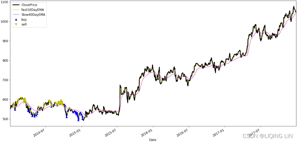
fig = plt.figure( figsize=(20,10) )

data4['APO'].plot( color='k', lw=3., legend=True )
plt.plot( data4.loc[ data4.Trades == 1 ].index, data4.APO[data4.Trades == 1 ],
          color='b', lw=0, marker='^', markersize=7, label='buy'
        )
plt.plot( data4.loc[ data4.Trades == -1 ].index, data4.APO[data4.Trades == -1 ],
          color='y', lw=0, marker='v', markersize=7, label='sell'
        )
plt.axhline(y=0, lw=0.5, color='k')
for i in range( APO_VALUE_FOR_BUY_ENTRY, APO_VALUE_FOR_BUY_ENTRY*5, APO_VALUE_FOR_BUY_ENTRY ):
  plt.axhline( y=i, lw=0.5, color='r' )
for i in range( APO_VALUE_FOR_SELL_ENTRY, APO_VALUE_FOR_SELL_ENTRY*5, APO_VALUE_FOR_SELL_ENTRY ):
  plt.axhline( y=i, lw=0.5, color='g' )

plt.autoscale(enable=True, axis='x', tight=True)
plt.legend()
plt.show()
The buy and sell trades that are overlaid on APO signal value changes also changed(
The higher the risk, the greater the possible return
)
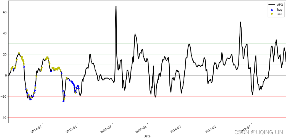
fig = plt.figure( figsize=(20,10) )

data4['Position'].plot(color='k', lw=1., legend=True)
plt.plot( data4.loc[ data4.Position == 0 ].index, data4.Position[ data4.Position == 0 ],
          color='r', lw=0, marker='.', label='flat'
        )
plt.plot( data4.loc[ data4.Position > 0 ].index, data4.Position[ data4.Position > 0 ],
          color='b', lw=0, marker='+', label='long'
        )
plt.plot( data4.loc[ data4.Position < 0 ].index, data4.Position[ data4.Position < 0 ],
          color='y', lw=0, marker='x', label='short'
        )
plt.axhline( y=0, lw=0.5, color='k')
plt.autoscale(enable=True, axis='x', tight=True)
plt.legend()
plt.show()
the position plot is especially interesting because it shows
how the magnitude of the positions increases over time
.
Initially, they are very small (less than 50 shares)
and increase or decrease or keep constant over time as strategy performance change :
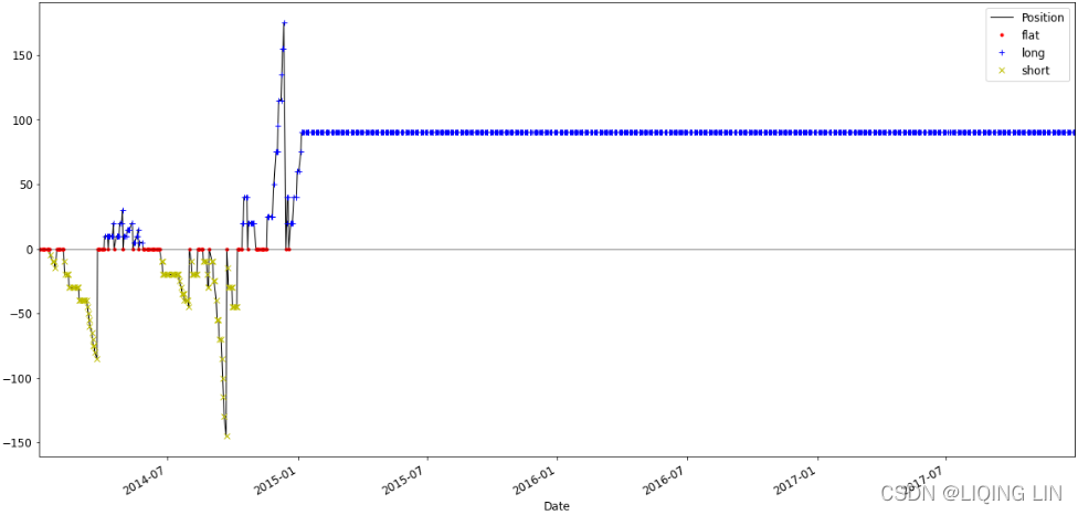
fig = plt.figure( figsize=(20,10) )

data4['Pnl'].plot(color='k', lw=1., legend=True)
plt.plot( data4.loc[ data4.Pnl > 0 ].index, data4.Pnl[ data4.Pnl > 0 ],
          color='b', lw=0, marker='.',
          label='Pnl'
        )
plt.plot( data4.loc[ data4.Pnl < 0 ].index, data4.Pnl[ data4.Pnl < 0 ],
          color='y', lw=0, marker='.',
          label='Pnl'
        )

plt.autoscale( enable=True, axis='x', tight=True)
plt.legend()
plt.show()
the
PnL plot
is also quite interesting and reflects what we would expect it to show. It slowly
increases initially when we are trading small sizes and over time
,
the trading sizes increase/decrease and the PnLs also increase/decrease with the larger change on trade size and risk limits
(check the following NumShares and MaxTradeSize plot)
:
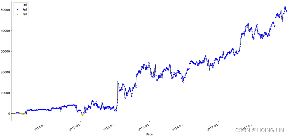
fig = plt.figure( figsize=(20,10) )

data4['NumShares'].plot( color='b', lw=3., legend=True )
data4['MaxTradeSize'].plot( color='y', lw=1., legend=True )
plt.autoscale( enable=True, axis='x', tight=True)
plt.legend()
plt.show()
the trade size and max trade size risk limit
evolution plot shows that, initially, we start with 5 share per trade, then increase it slowly when we have a positive month, then decrease it slowly when we have a negative month. In some periods(for example, from 2017-01 to 2017-04), the strategy gets into a streak of consecutively profitable months and causes
the trade size to increase every month
:
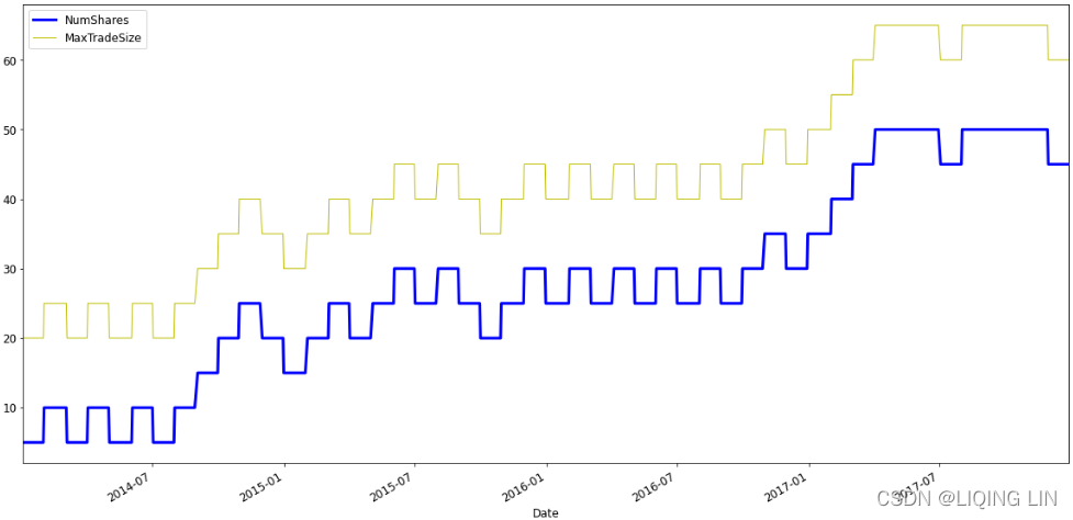
fig = plt.figure( figsize=(20,10) )

data4['AbsPosition'].plot( color='b', lw=1., legend=True )
data4['MaxPosition'].plot( color='g', lw=1., legend=True )
plt.autoscale( enable=True, axis='x', tight=True )
plt.legend()
plt.show()
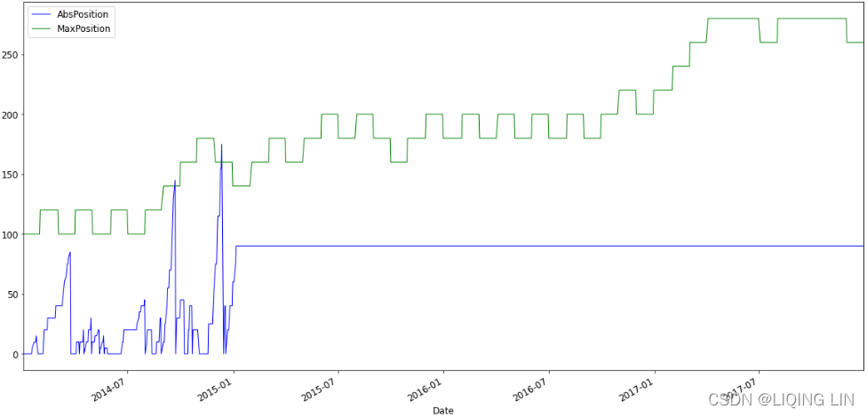
As shown in the preceding plot,
the
absolute positions that the strategy puts on
, as well as
the
max position risk limit evolution plot
, stay consistent with expectations, that is, starting low and then increase/decrease and even keep constant.
Summary
In this chapter, you learned about the
different types of risks and risk factors
. Then, we went through the sources of risk and learned about quantifying the risks. Moving ahead, we also learned about how to measure and
manage the risks (market risk, operational risk, and software implementation bugs) of algorithmic strategies
. We incorporated a full production-ready risk management system into our previously built trading strategy, thus making them safe for deployment to live trading markets. Finally, we discussed and built a practical risk scaling
system that starts with very low-risk exposure and dynamically manages the risk exposure over time as the strategy performance evolves
.
In the next chapter, we will look at how the algorithm’s trading interacts with the different factors in the trading arena. You will learn how to build a trading bot from scratch. Using the algorithm that we will build in the prior sections, you will know how to implement it, where to connect it, and how to handle it.