自然语言概念
自然语言,即我们人类日常所使用的语言,是人类交际的重要方式,也是人类区别于其他动物的本质特征。
我们只能使用自然语言与人进行交流,而无法与计算机进行交流。
自然语言处理
自然语言处理(NLP Natural Language Processing),是人工智能(AI Artificial Intelligence)的一部分,实现人与计算机之间的有效通信。
自然语言处理属于计算机科学领域与人工智能领域,其研究使用计算机编程来处理与理解人类的语言。
应用场景
自然语言处理,具有非常广泛的应用场景,例如:
- 情感分析
- 机器翻译
- 文本相似度匹配
- 智能客服
- 通用技术
- 分词
- 停用词过滤
- 词干提取
- 词形还原
- 词袋模型
- TF-IDF
- Word2Vec
说明:
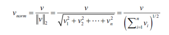
scikit-learn库中实现的tf-idf转换,与标准的公式略有不同。并且,tf-idf结果会使用L2范数进行规范化处理。
import numpy as np
# 对语料库中出现的词汇进行词频统计,相当于词袋模型。
# 操作方式:将语料库当中出现的词汇作为特征,将词汇在当前文档中出现的频率(次数)
# 作为特征值。
from sklearn.feature_extraction.text import CountVectorizer
count = CountVectorizer()
# 语料库
docs = np.array([
    "Where there is a will, there is a way.",
    "There is no royal road to learning.",
])
# bag是一个稀疏的矩阵。因为词袋模型就是一种稀疏的表示。
bag = count.fit_transform(docs)
# 输出单词与编号的映射关系。
print(count.vocabulary_)
# 调用稀疏矩阵的toarray方法,将稀疏矩阵转换为ndarray对象。
print(bag.toarray())
{'where': 8, 'there': 5, 'is': 0, 'will': 9, 'way': 7, 'no': 2, 'royal': 4, 'road': 3, 'to': 6, 'learning': 1}
[[2 0 0 0 0 2 0 1 1 1]
 [1 1 1 1 1 1 1 0 0 0]]
from sklearn.feature_extraction.text import TfidfTransformer
tfidf = TfidfTransformer()
print(tfidf.fit_transform(count.fit_transform(docs)).toarray())
[[0.53594084 0.         0.         0.         0.         0.53594084
  0.         0.37662308 0.37662308 0.37662308]
 [0.29017021 0.4078241  0.4078241  0.4078241  0.4078241  0.29017021
  0.4078241  0.         0.         0.        ]]
评论情感分析
项目背景
公司活动,新闻,微博,影评,商品评价等。
加载数据集
import pandas as pd
import numpy as np

data = pd.read_csv(r"movie.csv")
data.head()
label	comment
0	pos	此英雄完全自给自足,没有任何超能力,自己造就自己,酷!科技以人为本,发展才是硬道理!
1	pos	如果一个男人嫌女人太聪明了,那一定是因为他自己还不够牛逼
2	pos	这是一个会搞笑,爱臭屁又喋喋不休的英雄噢!结尾那句“I am Iron Man”太帅了~~
3	pos	没想到会比这侠那侠的都要好看!2个多小时的片子并不觉长,紧凑,爽快,意犹未尽……
4	pos	想起一个人,铁臂阿木童.
数据预处理
数据清洗
# 缺失值探索。
data.isnull().sum(axis=0)
# 异常值探索。
data["label"].value_counts()
# 重复值
# data.duplicated().sum()
# data[data.duplicated()]
data.drop_duplicates(inplace=True)
数据转换
将label与comment列转换为数值类型。
data["label"] = data["label"].map({"pos": 1, "neg": 0})

data["label"].value_counts()
1    11555
0     3928
Name: label, dtype: int64
# 用于进行中文分词的库。安装:
# pip install jieba

import jieba
import re

# 获取停用词列表
def get_stopword():
    # 默认情况下,在读取文件时,双引号会被解析为特殊的引用符号。双引号中的内容会正确解析,但是双引号不会解析为文本内容。
    # 在这种情况下,如果文本中仅含有一个双引号,会产生解析错误。如果需要将双引号作为普通的字符解析,将quoting参数设置为3。
    stopword = pd.read_csv(r"stopword.txt", header=None, quoting=3, sep="a")
    # 转换为set,这样可以比list具有更快的查询速度。
    return set(stopword[0].tolist())

# 清洗文本数据
def clear(text):
    return re.sub("[\s+\.\!\/_,$%^*(+\"\']+|[+——!,。?、~@#¥%……&*()]+", "", text)

# 进行分词的函数。
def cut_word(text):
    return jieba.cut(text)

# 去掉停用词函数。
def remove_stopword(words):
    # 获取停用词列表。
    stopword = get_stopword()
    return [word for word in words if word not in stopword]

def preprocess(text):
    # 文本清洗。
    text = clear(text)
    # 分词。
    word_iter = cut_word(text)
    # 去除停用词。
    word_list = remove_stopword(word_iter)
    return " ".join(word_list)

# 对文本数据(评论数据)的处理。步骤:
# 1 文本清洗。去掉一些特殊无用的符号,例如@,#。
# 2 分词,将文本分解为若干单词。
# 3 去除停用词。

# 以上步骤通过调用preprocess方法来实现。
data["comment"] = data["comment"].apply(lambda text: preprocess(text))
# 调用cut方法可以对文本进行分词,返回结果。cut方法返回的是生成器对象。
# jieba.cut("今天我们学习自然语言处理。")
# lcut方法返回的是列表。
# jieba.lcut("今天我们学习自然语言处理。")
data["comment"].head()
0             英雄 自给自足 超能力 造就 酷 科技 以人为本 发展 硬道理
1                        男人 嫌 女人 太 聪明 是因为 牛 逼
2    这是 搞笑 爱 臭屁 喋喋不休 英雄 噢 结尾 那句 IamIronMan 太帅
3         没想到 这侠 那侠 要好看 小时 片子 不觉 长 紧凑 爽快 意犹未尽
4                                   想起 铁臂 阿木童
Name: comment, dtype: object
# 使用TfidfVectorizer来进行文本向量化,具有一个局限(不足):就是语料库中存在多少个单词,就会具有多少个特征,
# 这样会造成特征矩阵非常庞大,矩阵非常稀疏。
from sklearn.feature_extraction.text import TfidfVectorizer
tfidf = TfidfVectorizer()
tfidf.fit_transform(data["comment"].tolist())
data["comment"]
0                          英雄 自给自足 超能力 造就 酷 科技 以人为本 发展 硬道理
1                                     男人 嫌 女人 太 聪明 是因为 牛 逼
2                 这是 搞笑 爱 臭屁 喋喋不休 英雄 噢 结尾 那句 IamIronMan 太帅
3                      没想到 这侠 那侠 要好看 小时 片子 不觉 长 紧凑 爽快 意犹未尽
4                                                想起 铁臂 阿木童
5                                                  个会 飞 锅炉
6                                          美国 人真 幼稚 喜欢 大力士
7        超级 英雄 电影 差 很远 RobertDowneyJr 天才 演员 电影 娱乐性 十足 话...
8                                            腐朽 堕落 资本主义 垃圾
9                                   爱看 商业片 动作片 科幻片 动画片 喜剧片
10                                        太拉风 装备 蝙蝠侠 摩托 拉风
11                                          资本主义 钢铁 炮弹 纸老虎
12                              蜘蛛侠 哈里波特 功夫 骇客帝国 攻壳 II 吐 死
13                                             真的 男生 喜欢 看吧
14                                                   高科技 份
15                                            中规中矩 超级 英雄 片
16                                                   侠中 算是
17       期望值 高 不免有些 失望 当作 minitransformer 斯坦 李 作品 名单 蜘蛛...
18                                             唐尼 goodluck
19                            复仇者 连门 回来 补 真的 片子 复仇者 联盟 啊啊啊
20                                                  Jarvis
21           主角 高 大帅 情节 老套 经不起 推敲 起伏跌宕 噱头 幽默 烂 装备 代表 票房 烂片
22       完 复仇者 联盟 倒 回来 第一部 发现 罗伯特 童孩 演了 福尔摩斯 特别 喜欢 咔 咔 ...
23                                          RobertDowneyJr
24                                             SEXYIRONMAN
25                                         电影院 看一看 图个 爽 片子
26                                            想 一套 钢铁 侠 铠甲
27                                               想起 铁臂 阿木童
28                                   视效 噱头 情节 弱得 要死 女一号 不错
29                                                 不错 人造 强
                               ...
15541                                        听 搞笑 研究 阶段 蛮牛
15542                             影片 没什么 兴趣 一部 超过 预期 值得 收藏
15543                迅雷 抢先 版画 质 差 总 找个 高清 版 弥补 情节 空洞 带给 失望
15544                                        昨天 钢铁 侠 感觉 不错
15545                                       灰常想 一套 钢铁 侠 衣服
15546                                            APPLESMOM
15547                                构思 错 动作 错 造型 很酷 故事 单调
15548                       comiccharactersuperhero fetish
15549    爱 marvel superhero 题材 电影 ironman 心理变态 小萝卜头 糖泥 ...
15550                                          赞 年 极力推荐 这部
15551    喜欢 美国 漫画 接触 机会 非常少 铁人 MARVEL 二线 英雄 电影 发现 错 仅次于...
15552                                         好看 我会 想起 奥特曼
15553                                             特效 不错 剧情
15554                                         美国式 英雄 场面 不错
15555    特效 不错 男人 心中 想 飞 冲动 男人 想 英雄 记住 喜欢 IRONMANSAY IA...
15556                      TONYSTARK 诙诣 语言 不错 那句 事实上 钢铁 侠帅
15557                                      电影 里 道具 科幻 构思新颖
15558                                 一部 好看 superheromovie
15559                                好看 电影 特地去 电影院 花 80 块钱
15560                                      08 年度 最棒 英雄 科幻片
15561              atypicalHolleywoodblockbusterNosurprise
15562                                     钢铁 侠 生活 完美 男人 生活
15563                                        不错 想象力 主角 牛 牛
15564          每次 美国 超级 英雄 电影 影虫们 失望 钢铁 侠 剧情 不谈 确实 场 视觉 盛宴
15565                                      不错 特别 组装 装甲 帅呆了
15566                                   诺 极力推荐 真的 失望 近期 好看
15567                                     目前为止 喜欢 超级 英雄 电影
15568                                              西 老公 喜欢
15569                              功夫 之王 烂片 强奸 强档 好片 回到 人间
15570                                   2008 04 30cathyAMK
Name: comment, Length: 15483, dtype: object
from sklearn.feature_extraction.text import TfidfVectorizer
from sklearn.model_selection import train_test_split
from sklearn.linear_model import LogisticRegression
from sklearn.pipeline import Pipeline
from sklearn.metrics import classification_report

X_train, X_test, y_train, y_test = train_test_split(data["comment"], data["label"], test_size=0.25, random_state=0)
# TfidfVectorizer可以看做是CountVectorizer与TfidfTransformer两个类型的合体。
tfidf = TfidfVectorizer()
lr = LogisticRegression(class_weight="balanced")
# lr = LogisticRegression()
steps = [("tfidf", tfidf), ("model", lr)]
pipe = Pipeline(steps=steps)
pipe.fit(X_train, y_train)
y_hat = pipe.predict(X_test)
print(pipe.score(X_train, y_train))
print(pipe.score(X_test, y_test))
print(classification_report(y_test, y_hat))
0.8405959352394075
0.672436063032808
              precision    recall  f1-score   support

           0       0.40      0.51      0.45      1004
           1       0.81      0.73      0.77      2867

   micro avg       0.67      0.67      0.67      3871
   macro avg       0.60      0.62      0.61      3871
weighted avg       0.70      0.67      0.68      3871
print(pd.Series(y_test).value_counts())
print(pd.Series(y_hat).value_counts())
1    2867
0    1004
Name: label, dtype: int64
1    2585
0    1286
dtype: int64
from sklearn.ensemble import RandomForestClassifier

rf = RandomForestClassifier(n_estimators=100, n_jobs=-1, class_weight="balanced")
# rf = RandomForestClassifier(n_estimators=100, n_jobs=-1)
pipe.set_params(model=rf)
pipe.fit(X_train, y_train)
y_hat = pipe.predict(X_test)
print(pipe.score(X_train, y_train))
print(pipe.score(X_test, y_test))
print(classification_report(y_test, y_hat))
0.9889769204271444
0.706277447687936
              precision    recall  f1-score   support

           0       0.38      0.21      0.27      1004
           1       0.76      0.88      0.82      2867

   micro avg       0.71      0.71      0.71      3871
   macro avg       0.57      0.55      0.54      3871
weighted avg       0.66      0.71      0.68      3871
from sklearn.ensemble import BaggingClassifier
from sklearn.tree import DecisionTreeClassifier

b = BaggingClassifier(base_estimator=DecisionTreeClassifier(), n_estimators=10, n_jobs=-1)
pipe.set_params(model=b)
pipe.fit(X_train, y_train)
y_hat = pipe.predict(X_test)
print(pipe.score(X_train, y_train))
print(pipe.score(X_test, y_test))
print(classification_report(y_test, y_hat))
0.9770065449534964
0.7091190906742444
              precision    recall  f1-score   support

           0       0.41      0.26      0.32      1004
           1       0.77      0.86      0.81      2867

   micro avg       0.71      0.71      0.71      3871
   macro avg       0.59      0.56      0.57      3871
weighted avg       0.68      0.71      0.69      3871
from sklearn.ensemble import AdaBoostClassifier

ada = AdaBoostClassifier(base_estimator=DecisionTreeClassifier(max_depth=1), n_estimators=100)
pipe.set_params(model=ada)
pipe.fit(X_train, y_train)
y_hat = pipe.predict(X_test)
print(pipe.score(X_train, y_train))
print(pipe.score(X_test, y_test))
print(classification_report(y_test, y_hat))
0.7695487426799862
0.7377938517179023
              precision    recall  f1-score   support

           0       0.48      0.13      0.21      1004
           1       0.76      0.95      0.84      2867

   micro avg       0.74      0.74      0.74      3871
   macro avg       0.62      0.54      0.52      3871
weighted avg       0.69      0.74      0.68      3871
版权声明:本文为R18830287035原创文章,遵循 CC 4.0 BY-SA 版权协议,转载请附上原文出处链接和本声明。